Call:
glm(formula = typeTF ~ glu, family = "binomial", data = Pima.te)

Deviance Residuals:
    Min       1Q   Median       3Q      Max
-2.2343  -0.7270  -0.4985   0.6663   2.3268

Coefficients:
             Estimate Std. Error z value Pr(>|z|)
(Intercept) -5.946808   0.659839  -9.013   <2e-16 ***
glu          0.042421   0.005165   8.213   <2e-16 ***
---
Signif. codes:  0 '***' 0.001 '**' 0.01 '*' 0.05 '.' 0.1 ' ' 1

(Dispersion parameter for binomial family taken to be 1)

    Null deviance: 420.30  on 331  degrees of freedom
Residual deviance: 325.99  on 330  degrees of freedom
AIC: 329.99

Number of Fisher Scoring iterations: 4
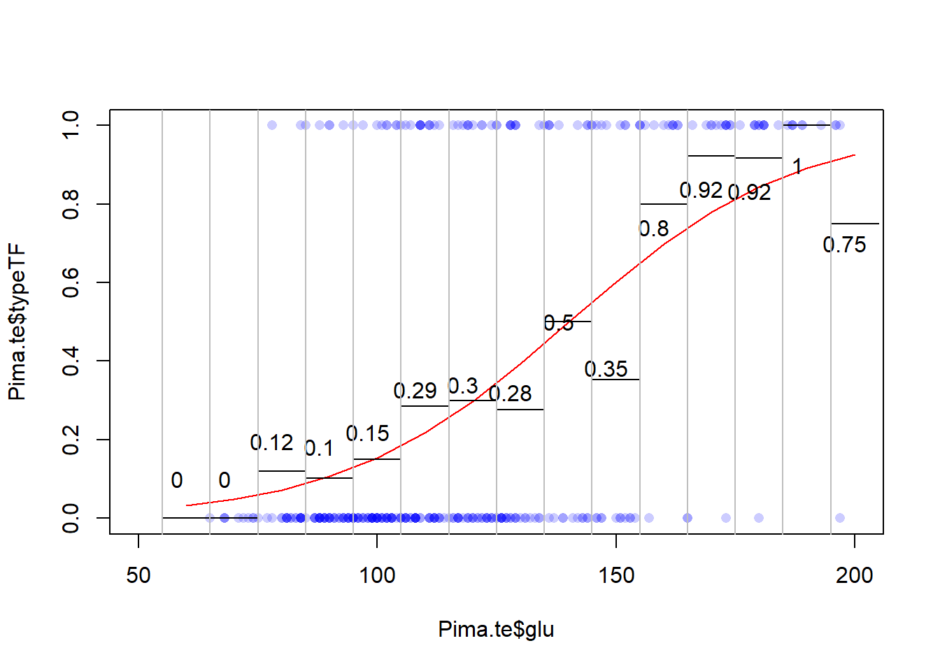
32.2 Odds Ratios
Odds Ratio = Odds(Event | Case A) / Odds(Event | Case B) We look at odds ratio when the cases differe by an increase of 1 unit in the predictor \(x\). \(\beta_1\) is the log of the odds ratio associated with a 1 unit increase in \(x\).
The log(odds ratio)=0.042421
The odds ratio = exp(0.042421)
exp(0.042421)
[1] 1.043334
32.2.1 Interpret the slope
Pima.glm$coefficients[2]
       glu
0.04242098
exp(Pima.glm$coefficients[2])
     glu
1.043334
Odd ratio for a 1 unit increase in blood glucose is 1.0433 so if we hold all other variables constant and increase blood glucose by 1 unit, we expect an increase in the Odds by 4.33%
32.2.2 odds ratio vs risk ratio
Risk is Prob(Event | case A) / Pr(Event | Case B) which is not the same as odds ratio. Consider this example:
The likelihood is the product of predicted probabilities (of the actual label) For actual 1s, we use y.hat For actual 0s we use 1-y.hat
L <-prod(y * y.hat + (1-y)*(1-y.hat))L
[1] 1.629075e-71
Maximizing likelihood is equivalent to maximising the log of likelihood, and because logarithms turn products into sums, the log likelihood is easier to work with mathematically. Because likelihood < 1, log likelihood is going to be negative.
log(L)
[1] -162.9955
l <-sum(log(y * y.hat + (1-y)*(1-y.hat)))l
[1] -162.9955
The closer to zero the log likelihood is, the better; The closer to -infinity, the “worse”.
The residual deviance is defined as -2 times the log likelihood. It turns a big negative log likelihood into a large positive number (easier to interpret)
#residual deviance-2*l
[1] 325.9911
For each observation, we can translate \(P(Y=y | model)\) into a log-likelihood by just taking the log of that decimal. Furthermore, we could multiply each of these by -2 to see which data points contribute more (or less) to the total “residual deviance”
The null model would be what we compare our “better” model to - it is a logistic model that does not have any predictors. Just like the null model for linear regression predicts \(\hat{y}=\bar{y}\) the null model predicts \(\hat{y}=\) the proportion of 1s in the data set.
Call:
glm(formula = typeTF ~ 1, family = "binomial", data = Pima.te)

Deviance Residuals:
    Min       1Q   Median       3Q      Max
-0.8921  -0.8921  -0.8921   1.4925   1.4925

Coefficients:
            Estimate Std. Error z value Pr(>|z|)
(Intercept)  -0.7158     0.1169  -6.125 9.07e-10 ***
---
Signif. codes:  0 '***' 0.001 '**' 0.01 '*' 0.05 '.' 0.1 ' ' 1

(Dispersion parameter for binomial family taken to be 1)

    Null deviance: 420.3  on 331  degrees of freedom
Residual deviance: 420.3  on 331  degrees of freedom
AIC: 422.3

Number of Fisher Scoring iterations: 4
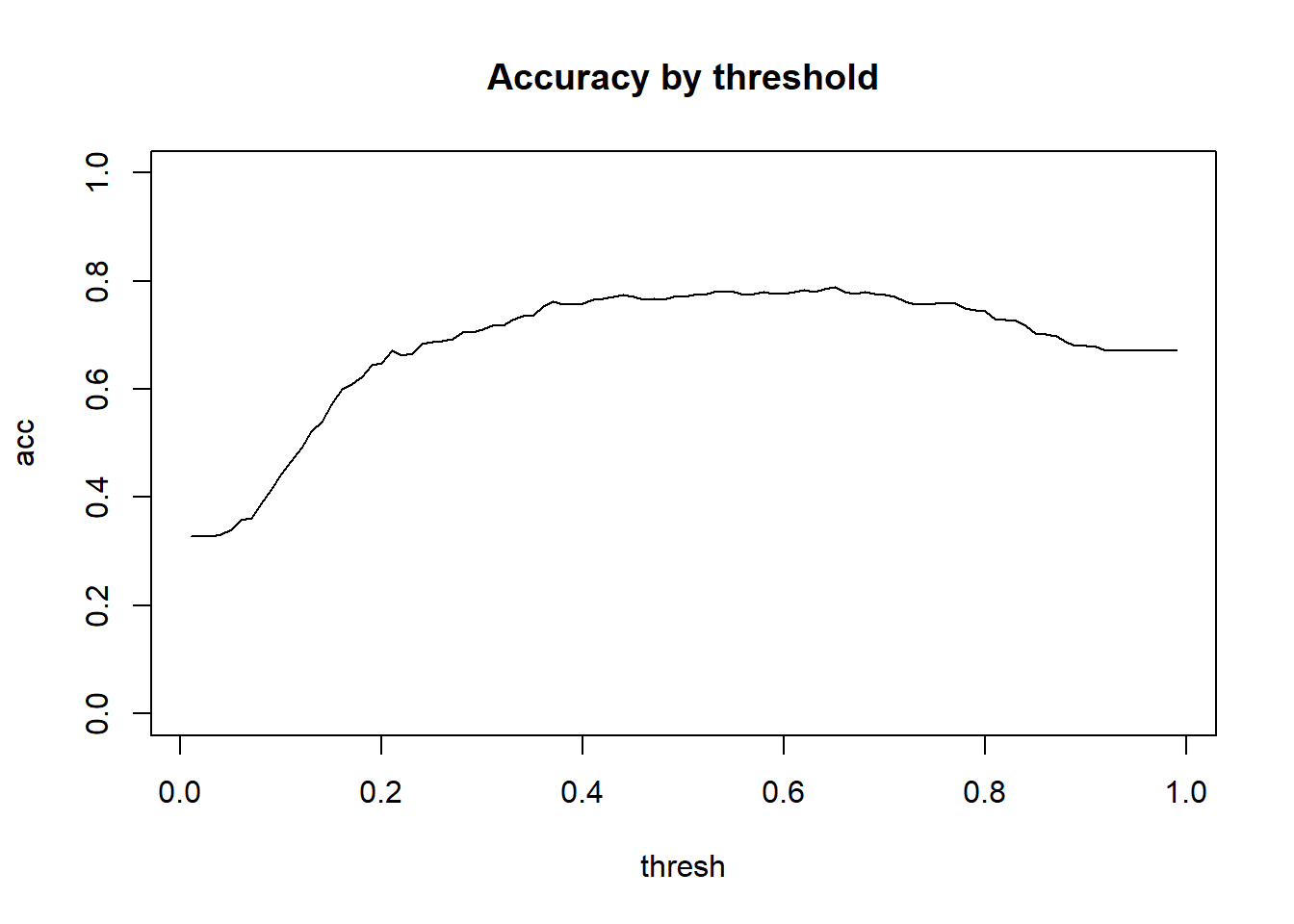
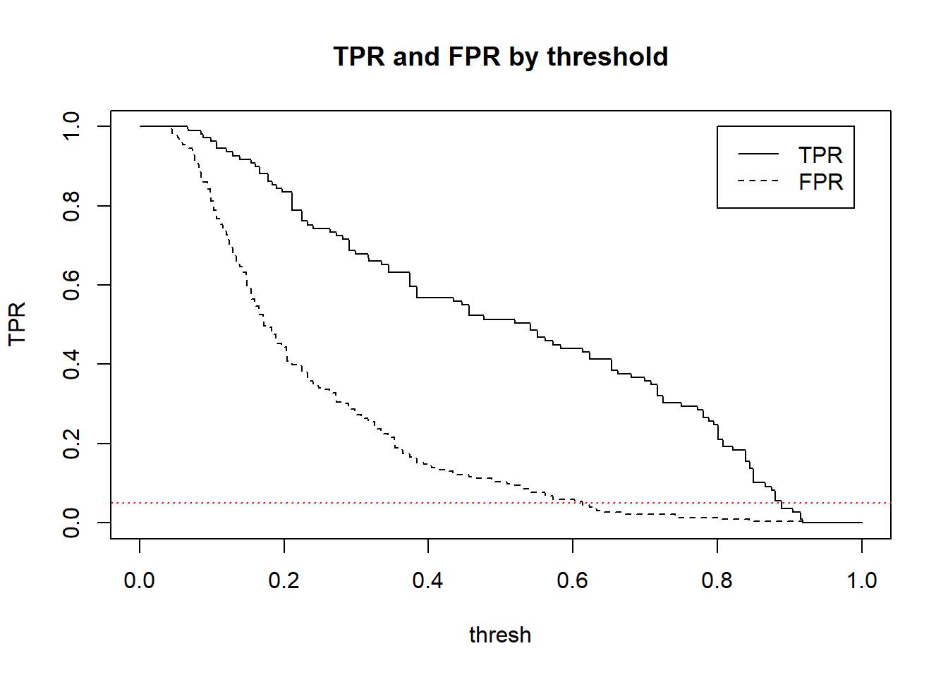
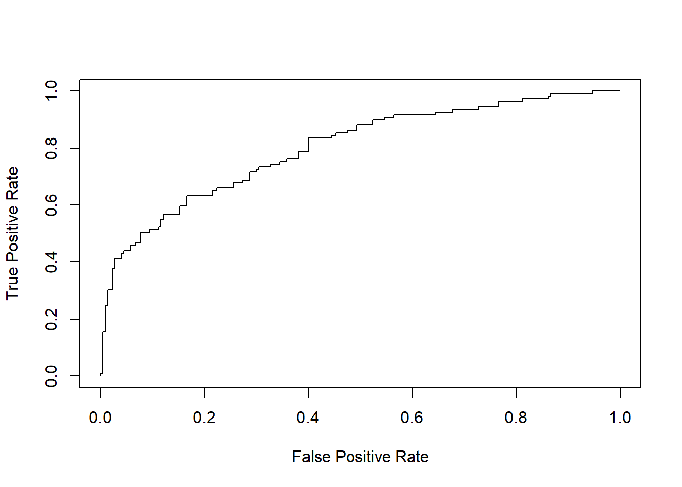
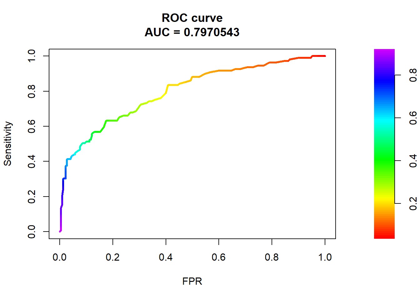
In particular, we can look at the relationship between True positive rate and False Positive Rate (what proportion of actual negatives are incorrectly predicted to be positive) (FP / (FP+TN))
To put things into the language of hypothesis testing we could ask this: What threshold would we use to achieve a 5% significance level (false positive rate) and what would the power of the classifier be?
The area under the curve (AUC) is a common metric measuring how good your classifier is. An AUC = 0.5 (where the ROC curve is a diagonal line) is a “dumb” predictor. AUC closer to 1 represents a discerning “good” predictor.
32.7 Comparing using AIC and BIC
As we’ll see next week, the AIC (Akaike Information Criterion) is a useful statistic to compare logistic models. \[AIC = \text{residual deviance} + 2k\text{ (k is the number of coefficients fit)}\]\[BIC = \text{residual deviance} + ln(n)*k\] When sample size is large then BIC will give a larger penalty per predictor. \(ln(8) > 2\) so when \(n \geq 8\) BIC gives a heftier penalty per coefficient in the model than AIC does and thus will favor simpler models.
When using either of these comparative statistics, the lower the value the better.
Call:
glm(formula = typeTF ~ 1 + glu, family = "binomial", data = Pima.te)

Deviance Residuals:
    Min       1Q   Median       3Q      Max
-2.2343  -0.7270  -0.4985   0.6663   2.3268

Coefficients:
             Estimate Std. Error z value Pr(>|z|)
(Intercept) -5.946808   0.659839  -9.013   <2e-16 ***
glu          0.042421   0.005165   8.213   <2e-16 ***
---
Signif. codes:  0 '***' 0.001 '**' 0.01 '*' 0.05 '.' 0.1 ' ' 1

(Dispersion parameter for binomial family taken to be 1)

    Null deviance: 420.30  on 331  degrees of freedom
Residual deviance: 325.99  on 330  degrees of freedom
AIC: 329.99

Number of Fisher Scoring iterations: 4
summary(pima.logit2)
Call:
glm(formula = typeTF ~ 1 + glu + bmi, family = "binomial", data = Pima.te)

Deviance Residuals:
    Min       1Q   Median       3Q      Max
-2.2240  -0.7216  -0.4421   0.6158   2.3544

Coefficients:
             Estimate Std. Error z value Pr(>|z|)
(Intercept) -8.025302   0.942896  -8.511  < 2e-16 ***
glu          0.039311   0.005257   7.478 7.57e-14 ***
bmi          0.072645   0.020621   3.523 0.000427 ***
---
Signif. codes:  0 '***' 0.001 '**' 0.01 '*' 0.05 '.' 0.1 ' ' 1

(Dispersion parameter for binomial family taken to be 1)

    Null deviance: 420.30  on 331  degrees of freedom
Residual deviance: 312.49  on 329  degrees of freedom
AIC: 318.49

Number of Fisher Scoring iterations: 4
32.8 Example 2: A Logistic model with a categorical predictor
#Let's use age as a predictor#Only for age > 50Pima.te$age50 <-as.numeric(Pima.te$age >50)diabetes.aggr <-aggregate(typeTF ~ age50, data=Pima.te, FUN=mean)diabetes.aggr
  age50    typeTF
1     0 0.3129032
2     1 0.5454545
Among those 50 or younger, proportion with diabetes is .3129032 among those 51+ it is .545454
#Log-odds for the two groupsodds <- diabetes.aggr$typeTF / (1-diabetes.aggr$typeTF)odds
[1] 0.4553991 1.2000000
logodds <-log(odds)logodds
[1] -0.7865812 0.1823216
diff(logodds)
[1] 0.9689027
Notice the log-odds are -.7865 and .1823 respectively. If we were to build a model we would say that \[ \hat{LO} = -.7865812 + .9689 \times age_{>50}\]
Call:
glm(formula = typeTF ~ age50, family = "binomial", data = Pima.te)

Deviance Residuals:
    Min       1Q   Median       3Q      Max
-1.2557  -0.8663  -0.8663   1.5244   1.5244

Coefficients:
            Estimate Std. Error z value Pr(>|z|)
(Intercept)  -0.7866     0.1225  -6.422 1.35e-10 ***
age50         0.9689     0.4454   2.176   0.0296 *
---
Signif. codes:  0 '***' 0.001 '**' 0.01 '*' 0.05 '.' 0.1 ' ' 1

(Dispersion parameter for binomial family taken to be 1)

    Null deviance: 420.30  on 331  degrees of freedom
Residual deviance: 415.59  on 330  degrees of freedom
AIC: 419.59

Number of Fisher Scoring iterations: 4
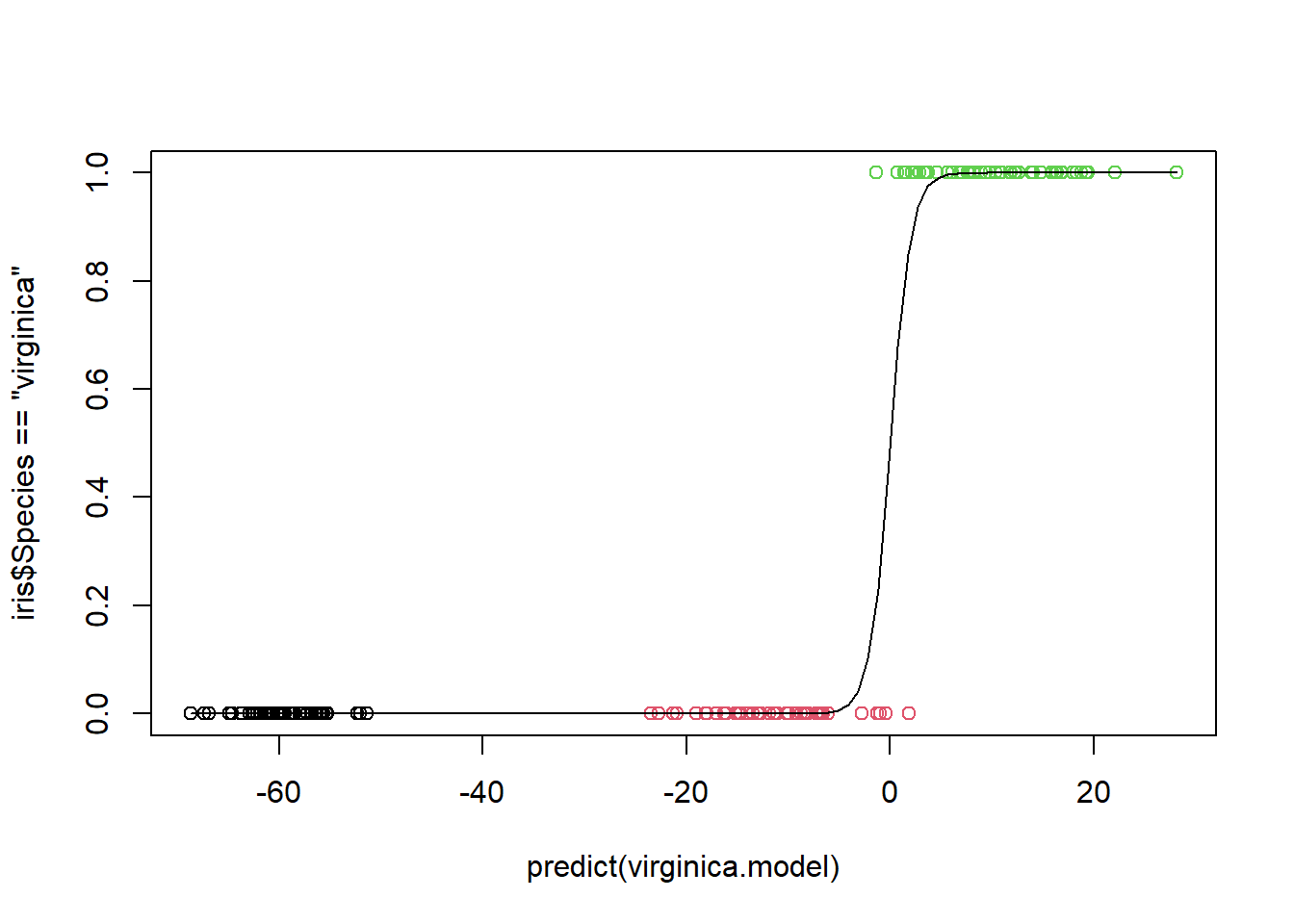
32.9 Example 3: Iris dataset
Another classic example is the iris dataset. This famous dataset gives measurements in centimeters of the sepal and petal width and length for 3 species of iris: setosa, versicolor and virginica. The dataset has 150 rows, with 50 samples of each.
Because the logistic model handles binary response variables, what we will do is create a logistic model to predict whether an iris is virginica Let’s build a full model with all 4 predictors.
Call:
glm(formula = Species == "virginica" ~ 1 + Sepal.Length, family = "binomial",
    data = iris)

Deviance Residuals:
    Min       1Q   Median       3Q      Max
-1.9870  -0.5520  -0.2614   0.5832   2.7001

Coefficients:
             Estimate Std. Error z value Pr(>|z|)
(Intercept)  -16.3198     2.6581  -6.140 8.27e-10 ***
Sepal.Length   2.5921     0.4316   6.006 1.90e-09 ***
---
Signif. codes:  0 '***' 0.001 '**' 0.01 '*' 0.05 '.' 0.1 ' ' 1

(Dispersion parameter for binomial family taken to be 1)

    Null deviance: 190.95  on 149  degrees of freedom
Residual deviance: 117.35  on 148  degrees of freedom
AIC: 121.35

Number of Fisher Scoring iterations: 5
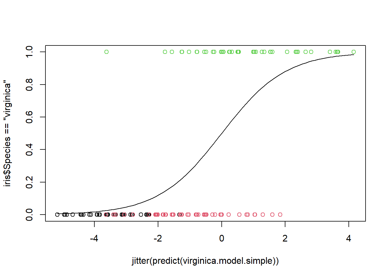
prop.table(table(predict =predict(virginica.model, type="response")>0.00504067 , actual = iris$Species=="virginica"), margin=2)
       actual
predict FALSE TRUE
  FALSE  0.95 0.00
  TRUE   0.05 1.00
We require very little evidence to claim the flower is virginica, a probability of 0.00504 is enough. In this case we have a 5% type 1 error rate. But note that the power has increased to 100%.
32.9.1 When a logistic model cannot converge
If your model is so good that it correctly labels everyhing as 1 or zero this is what the output looks like
Warning: glm.fit: fitted probabilities numerically 0 or 1 occurred
summary(setosa.model)
Call:
glm(formula = Species == "setosa" ~ 1 + Sepal.Length + Sepal.Width +
    Petal.Length + Petal.Width, family = "binomial", data = iris)

Deviance Residuals:
       Min          1Q      Median          3Q         Max
-3.185e-05  -2.100e-08  -2.100e-08   2.100e-08   3.173e-05

Coefficients:
               Estimate Std. Error z value Pr(>|z|)
(Intercept)     -16.946 457457.106       0        1
Sepal.Length     11.759 130504.043       0        1
Sepal.Width       7.842  59415.386       0        1
Petal.Length    -20.088 107724.596       0        1
Petal.Width     -21.608 154350.619       0        1

(Dispersion parameter for binomial family taken to be 1)

    Null deviance: 1.9095e+02  on 149  degrees of freedom
Residual deviance: 3.2940e-09  on 145  degrees of freedom
AIC: 10

Number of Fisher Scoring iterations: 25
It means that the coefficients are able to separate the predicted log odds so far that you have no misclassifications. Note above that after 25 fisher iterations it stopped. You can set the max iterations to be a lot lower, like 3, and then the model summary will be far more interpretable. But the standard errors of the coefficients will still be high so you can’t say much about the significance of individual predictors.
setosa.model.maxit <-glm(Species=="setosa"~1+ Sepal.Length + Sepal.Width+Petal.Length+Petal.Width, data=iris, family="binomial", control =list(maxit =2))
Warning: glm.fit: algorithm did not converge
summary(setosa.model.maxit)
Call:
glm(formula = Species == "setosa" ~ 1 + Sepal.Length + Sepal.Width +
    Petal.Length + Petal.Width, family = "binomial", data = iris,
    control = list(maxit = 2))

Deviance Residuals:
    Min       1Q   Median       3Q      Max
-0.7003  -0.2994  -0.1592   0.2188   0.7140

Coefficients:
             Estimate Std. Error z value Pr(>|z|)
(Intercept)   -2.4428     3.1506  -0.775   0.4381
Sepal.Length   0.4038     0.8871   0.455   0.6490
Sepal.Width    1.8157     0.8944   2.030   0.0424 *
Petal.Length  -1.7249     0.8993  -1.918   0.0551 .
Petal.Width   -0.2378     1.5787  -0.151   0.8803
---
Signif. codes:  0 '***' 0.001 '**' 0.01 '*' 0.05 '.' 0.1 ' ' 1

(Dispersion parameter for binomial family taken to be 1)

    Null deviance: 190.954  on 149  degrees of freedom
Residual deviance:  14.313  on 145  degrees of freedom
AIC: 24.313

Number of Fisher Scoring iterations: 2