27  Simple Linear Regression Practice

28 Practice Problems

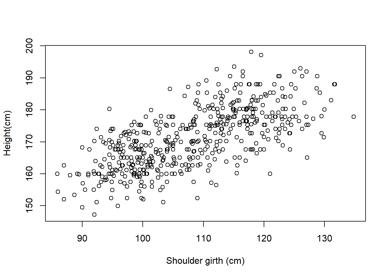
1. Researchers studying anthropometry collected body and skeletal diameter measurements, as well as age, weight, height and sex for 507 physically active individuals. The scatterplot below shows the relationship between height and shoulder girth (circumference of shoulders measured over deltoid muscles), both measured in centimeters.

if(!require(openintro)){
install.packages("openintro")
library(openintro)
}

Loading required package: openintro

Loading required package: airports

Loading required package: cherryblossom

Loading required package: usdata

plot(x=bdims$sho_gi, y=bdims$hgt, xlab="Shoulder girth (cm)", ylab = "Height(cm)")

1. Describe the relationship between shoulder girth and height.

Solution

There is a positive, seemingly linear relationship between shoulder girth and height. It seems to be a moderately strong association.

2. How would the relationship change if shoulder girth was measured in inches while the units of height remained in centimeters?

Solution

The relationship would be the same if the units of shoulder girth were changed; the only change to the plot would be the labeling of the X axis. The scatterplot itself would appear unchanged.

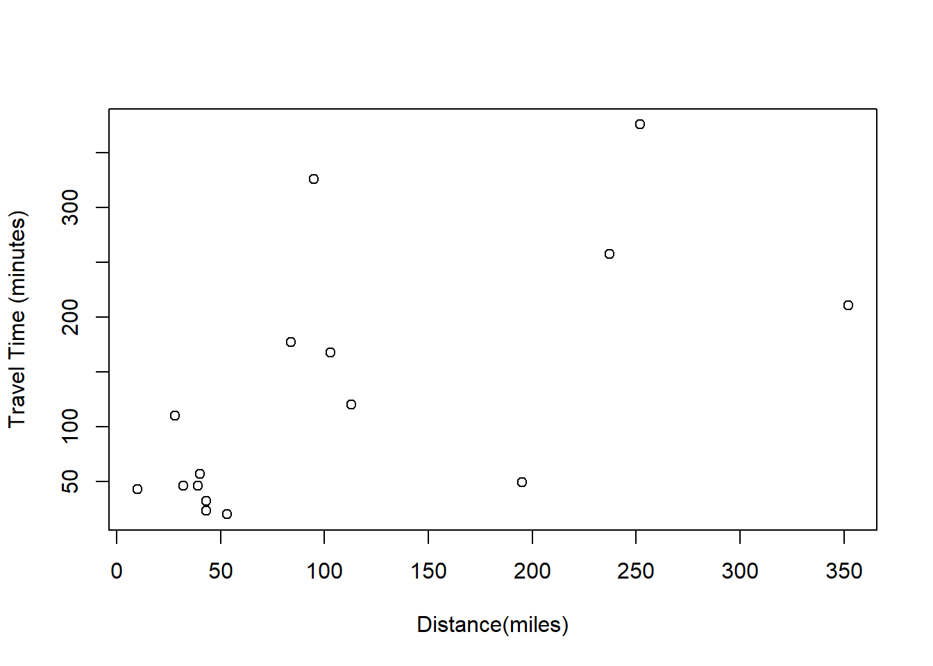
2. The Coast Starlight Amtrak train runs from Seattle to Los Angeles. The scatterplot below displays the distance between each stop (in miles) and the amount of time it takes to travel from one stop to another (in minutes).

Solution

plot(x=coast_starlight$dist, y=coast_starlight$travel_time, xlab="Distance(miles)", ylab="Travel Time (minutes)")

1. Describe the relationship between distance and travel time.

Solution

As distance tends to increase the travel time tends to increase as well, but there is a great deal of variability.

2. How would the relationship change if travel time was instead measured in hours, and distance was instead measured in kilometers?

Solution

If the units were changed linearly (miles to km, and minutes to hours) the association would not be affected.

3. Correlation between travel time (in miles) and distance (in minutes) is r = 0.636. What is the correlation between travel time (in kilometers) and distance (in hours)?

Solution

The correlation between travel time in km and distance in hours would be the exact same as the correlation with the original units. Correlation is a standardized statistic and is unaffected by affine (linear) transformations in the variables.

4. Write the equation of the regression line for predicting travel time.

Solution

starlight.lm <- lm(travel_time ~ 1 + dist, data=coast_starlight)
starlight.lm

Call:
lm(formula = travel_time ~ 1 + dist, data = coast_starlight)

Coefficients:
(Intercept)         dist  
    50.8842       0.7259  

The predicted model is \(\hat{time} = 50.8842 + 0.7259\cdot dist\)

5. Interpret the slope and the intercept in this context.

Solution

The slope can be interpreted as the average increase in travel time (.7259 minutes) for a 1 mile increase in travel distance. The slope does not have a meaningful interpretation as a zero distance trip would not take 50.88 minutes.

6. Calculate \(R^2\) of the regression line for predicting travel time from distance traveled for the Coast Starlight, and interpret \(R^2\) in the context of the application.

Solution

summary(starlight.lm)$r.sq

[1] 0.4044083

The \(R^2\) statistic equals 0.4044, which can be interpreted as variation in travel distance accounts for 40.44% of the variation in travel time along the Amtrak Starlight train line.

7. The distance between Santa Barbara and Los Angeles is 103 miles. Use the model to estimate the time it takes for the Starlight to travel between these two cities.

Solution

sum(coef(starlight.lm)*c(1, 103))

[1] 125.6537

#or
predict(starlight.lm, newdata=data.frame(dist=103))

       1 
125.6537 

Using our model we would predict the travel time between Santa Barbara and Los Angeles to be 125.65 minutes.

8. It actually takes the Coast Starlight about 168 mins to travel from Santa Barbara to Los Angeles. Calculate the residual and explain the meaning of this residual value.

Solution

168 - 125.65

[1] 42.35

The residual is 42.35 minutes; That means that our model under-estimates the travel time between Santa Barbara and Los Angeles by 42.35 minutes.

1. Suppose Amtrak is considering adding a stop to the Coast Starlight 500 miles away from Los Angeles. Would it be appropriate to use this linear model to predict the travel time from Los Angeles to this point?

Solution

range(coast_starlight$dist)

[1]  10 352

Because the dataset that generated this model included distances from 10 to 352 miles, it would only be appropriate to use this model to predict travel time for distances in this range. We lack any evidence from the dataset that the modeled relationship exists for distances beyond 352 miles.

3. What would be the correlation between the ages of partners if people always dated others who are

1. 3 years younger than themselves?

Solution

The correlation would be positive, it would be close to 1.

age.a <- runif(1000,40,100)
age.b <- age.a -3
cor(age.a, age.b)

[1] 1

2. 2 years older than themselves?

Solution

The correlation would be positive, close to 1.

age.a <- runif(1000,40,100)
age.b <- age.a +2
cor(age.a, age.b)

[1] 1

3. half as old as themselves?

Solution

The correlation would be positive, and it would again be close to 1.

age.a <- runif(1000,40,100)
age.b <- age.a / 2
cor(age.a, age.b)

[1] 1

4. Suppose we fit a regression line to predict the shelf life of an apple based on its weight. For a particular apple, we predict the shelf life to be 4.6 days. The apple’s residual is -0.6 days. Did we over or under estimate the shelf-life of the apple? Explain your reasoning.

Solution

The residual is \(y-\hat{y}\) or \(observed-predicted\). A negative residual indicates that \(\hat{y} > y\), so our model would have over-estimated shelf life for this apple.

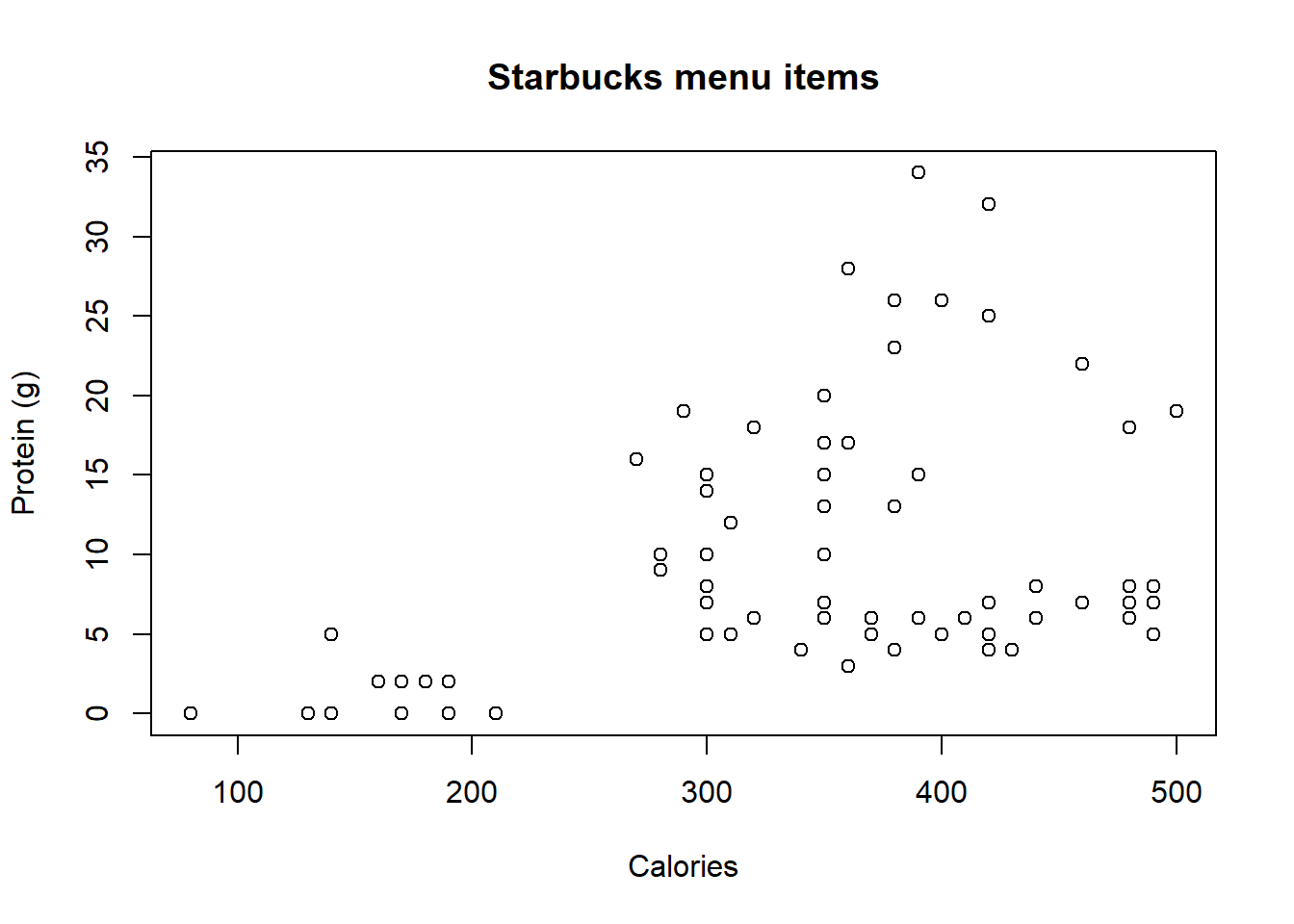
5. Explore the starbucks dataset in the openintro package, specifically the relationship between the number of calories and the amount of protein (in grams) in Starbucks food. Since Starbucks only lists the number of calories on the display items, we might be interested in predicting the amount of protein a menu item has based on its calorie content.

1. Create a scatter plot with protein as the Y variable and calories as the X variable.

Solution

plot(y=starbucks$protein, x=starbucks$calories, xlab="Calories", ylab="Protein (g)", main="Starbucks menu items")

2. Describe the relationship between number of calories and amount of protein (in grams) that Starbucks food menu items contain. b.

Solution

There is a general trend that foods with higher calorie levels tend to have higher amounts of protein, but there is a great deal of variability. The positive trend is apparent though.

3. In this scenario, what are the predictor and outcome variables

Solution

The predictor variable is calories, since that is the one piece of information labeled on the menu items. The outcome variable is protien (g), since we would try to predict that based on calories.

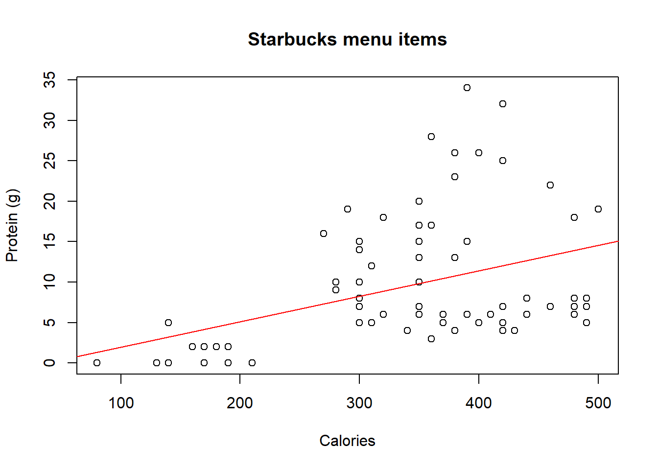
4. Why might we want to fit a regression line to these data?

Solution

The relationship between calories and protein seems like it might be linear, and a straight relationshup lends itself to OLS regression.

5. The following linear model is fit to the data:

starbucks.lm <- lm(protein ~ 1 + calories, data=starbucks)
plot(y=starbucks$protein, x=starbucks$calories, xlab="Calories", ylab="Protein (g)", main="Starbucks menu items")
abline(starbucks.lm, col="red")

plot(starbucks.lm, which=1)

\(\hat{protein} = -1.18211 + 0.03147 \cdot calories\)

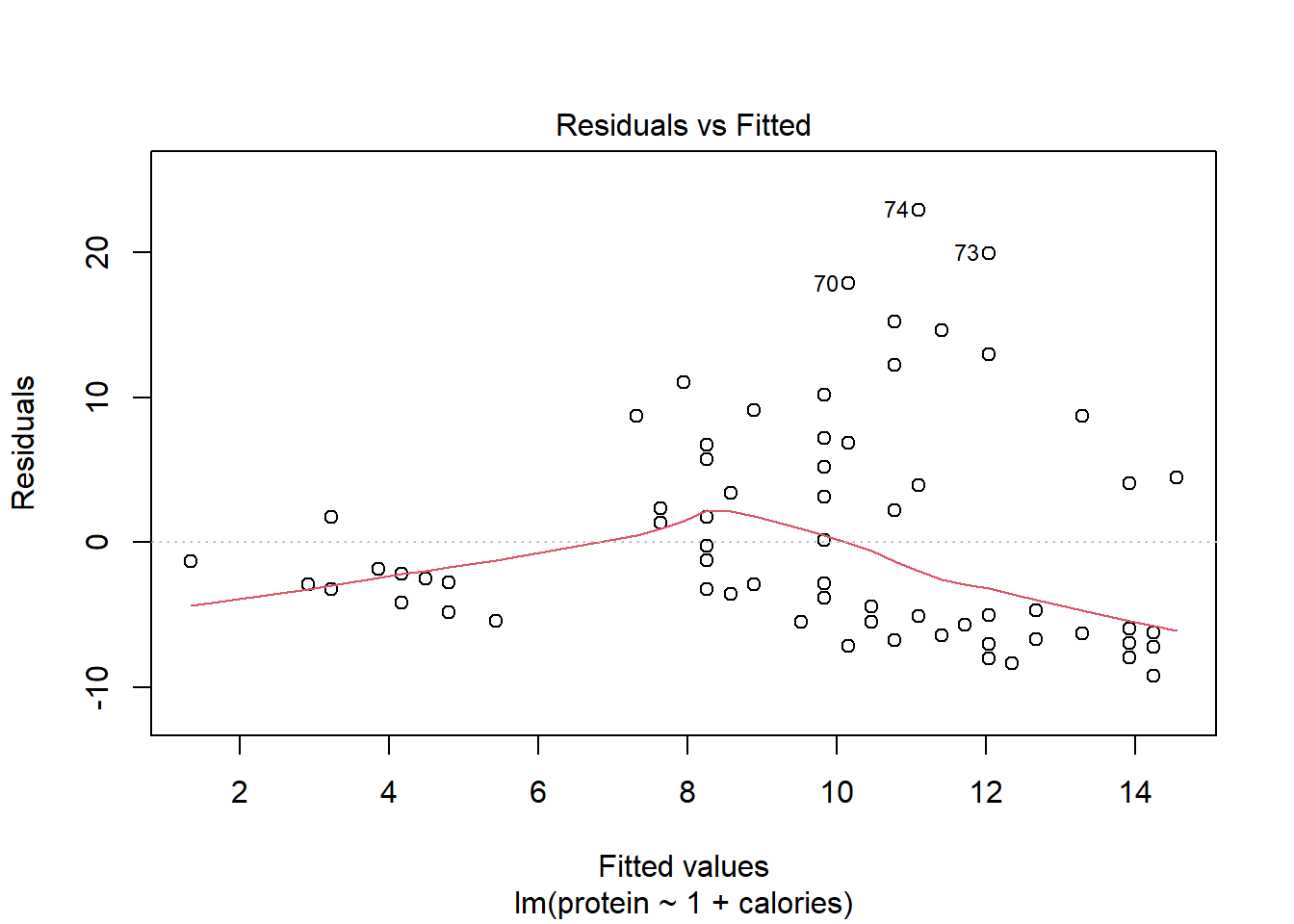
What does the residuals vs. predicted plot tell us about the variability in our prediction errors based on this model for items with lower vs. higher predicted protein?

Solution

This plot demonstrates very clearly that the variability is not constant; we have much higher variation in protein for foods with higher predicted protein than in foods with lower predicted protein. This indicates a violation in the assumption of constant variance. In order to fit a linear model perhaps the data should be transformed first, for example a log-transformation to the variables.

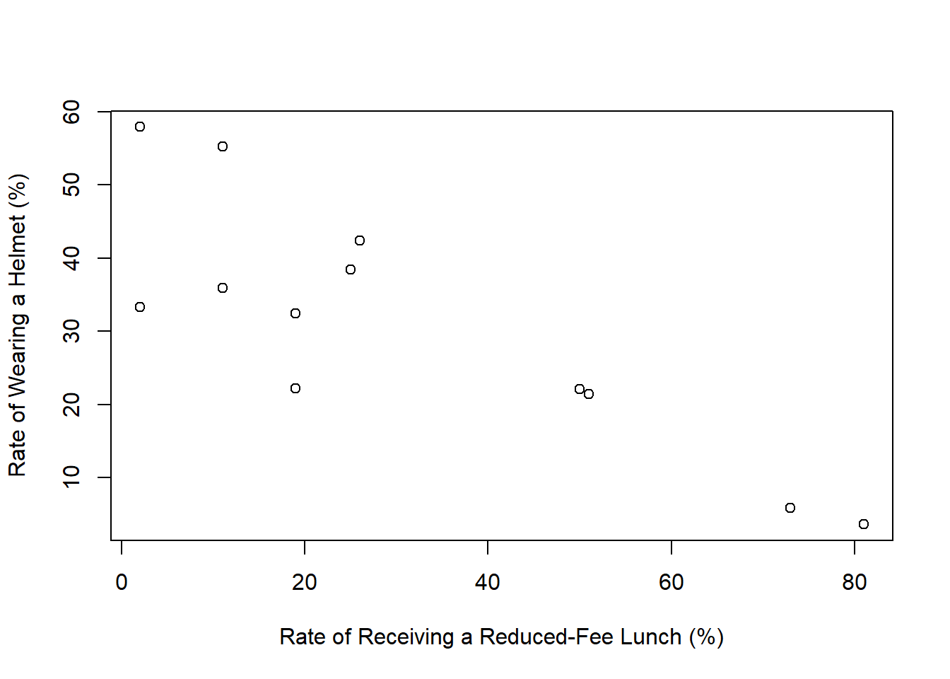
6. The scatterplot shows the relationship between socioeconomic status measured as the percentage of children in a neighborhood receiving reduced-fee lunches at school (lunch) and the percentage of bike riders in the neighborhood wearing helmets (helmet). The average percentage of children receiving reduced-fee lunches is 30.833% with a standard deviation of 26.724% and the average percentage of bike riders wearing helmets is 30.883% with a standard deviation of 16.948%.

library(openintro)
plot(helmet$helmet ~ helmet$lunch, xlab="Rate of Receiving a Reduced-Fee Lunch (%)", ylab="Rate of Wearing a Helmet (%)")

1. If the \(R^2\) for the least-squares regression line for these data is 72%, what is the correlation between lunch and helmet?

Solution

Correlation is precisely the square root of \(R^2\), the coefficient of determination. Therefore, the correlation would be

sqrt(.72)

[1] 0.8485281

2. Calculate the slope and intercept for the least-squares regression line for these data.

Solution

helmet.lm <- lm(helmet ~ lunch, data=helmet)
coef(helmet.lm)

(Intercept)       lunch 
 47.4904464  -0.5386091 

The slope is -.5386 and the intercept is 47.49.

3. Interpret the intercept of the least-squares regression line in the context of the application.

Solution

The intercept would be interpreted that in a neighborhood where 0% of the children receive reduced fare lunches, we predict that 47.49% of bike riders wear helmets.

4. Interpret the slope of the least-squares regression line in the context of the application.

Solution

For every percentage point increase in rate of children receiving reduced fare lunches, we predict the rate of bike-riders who wear helmets to decrease on average by 0.5386 percentage points.

5. What would the value of the residual be for a neighborhood where 40% of the children receive reduced-fee lunches and 40% of the bike riders wear helmets? Interpret the meaning of this residual in the context of the application.

Solution

40-predict(helmet.lm, newdata=data.frame(lunch=40))

       1 
14.05392 

The residual comes to 14.05392, which means our model under-estimates the helmet rate in this neighborhood by 14.04392 percentage points.

29 Beyond STAT 340

These problems are excellent practice but they are beyond the material we cover in STAT 340.