generate_data <- function(n){
  X <- rnorm(n, 5, 4)
  eps <- rnorm(n, 0, 2)
  Y <- 10 + 2*X + eps
  return(data.frame(X,Y))
}36 Bias Variance Tradeoff
36.1 Bias and Variance of an Linear Model
We will sample from a population, fit a linear model, then predict 1000 data points. We will actually repeat this over and over and in the end we will have 1000 model fits and for each one we will have 1000 predictions.
The true model is
\[Y_i = 10 + 2X_i + \epsilon_i, \text{ where }\epsilon\sim N(0,2^2)\] A simple function will be used to generate an unlimited number of data so we can precisely estimate out of sample error for our model.
The question is this: What is the expected model error of this linear model based on a sample size of 32, for this population? We’ll start with 1000 out of sample data points, which we can take as being representative of the population of out of sample data.
For 1000 Monte Carlo replicates we’ll
- Generate a random sample of size 32
- Fit a linear model to the data
- Make predictions for all 1000 out of sample data
- Calculate the average squared error on those predictions
This will give us a great estimate of model error. We can then use this as a benchmark for K-fold cross validation in the next phase of this example.
Note: This code can take a little bit to run
NMC <- 1000
nOut <- 1000
outData <- generate_data(nOut)

results <- data.frame('rep' = rep(1:NMC, nOut),
                      'i' = rep(1:nOut, each=NMC),
                      'X' = rep(outData$X, each=NMC),
                      'Y' = rep(outData$Y, each=NMC),
                      'beta0' = rep(0,nOut*NMC),
                      'beta1' = rep(0,nOut*NMC),
                      'Yhat' = rep(0,nOut*NMC),
                      'error'= rep(0,nOut*NMC))

for(k in 1:NMC){
  sampleData <- generate_data(32)
  modelFit <- lm(Y~X, data=sampleData)
  yhat <- predict(modelFit, newdata=outData)
  results[results$rep==k, "beta0"] <- coef(modelFit)[1]
  results[results$rep==k, "beta1"] <- coef(modelFit)[2]
  results[results$rep==k,"Yhat"] <- yhat
}
results$error = results$Y-results$Yhat

predVar <- as.numeric(mean(aggregate(error~rep, results, FUN="var")$error))
predBias2 <- mean(aggregate(error~rep, results, FUN="mean")$error)^2
predErr <- mean(results$error^2)
Variance of predictions is 3.883823.
Squared Bias of predictions is 0.0104627.
Mean Square Error is 4.0225088
Var + Bias^2 = 3.8942857.
A great explanation of the Bias Variance Tradeoff
NMC <- 500
ks <- c(2,4,8,16,32)
crossValidationResults <- data.frame('k' = ks,
                                     trainingError = 0,
                                     testingError = 0,
                                     testingVariance = 0,
                                     testingBias2 = 0,
                                     estimationError=0)

for(K in ks){
  trnErr <- 0
  tstErr <- 0

  for(j in 1:NMC){
    set.seed(j) #same data, repeated once for each k
    sampleData <- generate_data(32)

    #idx is a shuffled vector of row numbers
    idx <- sample(1:nrow(sampleData))
    #folds partitions the row indices
    folds <- split(idx, as.factor(1:K))

    trainingErrors <- 0
    testingErrors <- 0

    for(k in 1:K){
      training <- sampleData[-folds[[k]],]
      testing <- sampleData[folds[[k]],]
      #estimate MSE
      #fit the model to the training data
      modelFit <- lm(Y~X, data=training)
      #calculate the average squared error on the testing data
      trainingErrors[k] <- mean(resid(modelFit)^2)
      testingErrors[k] <- mean((predict(modelFit, newdata=testing) - testing$Y)^2)
    }

    trnErr[j] <- mean(trainingErrors)
    tstErr[j] <- mean(testingErrors)
  }
  crossValidationResults[crossValidationResults$k==K, "trainingError"] <- mean(trnErr)
  crossValidationResults[crossValidationResults$k==K, "testingError"] <- mean(tstErr)

  crossValidationResults[crossValidationResults$k==K, "testingVariance"] <- var(tstErr)
  crossValidationResults[crossValidationResults$k==K, "testingBias2"] <- mean((tstErr-4))^2
  crossValidationResults[crossValidationResults$k==K, "estimationError"] <- mean((tstErr-4)^2)
}
crossValidationResults
k trainingError testingError testingVariance testingBias2 estimationError
1 2 3.477456 4.498287 1.992548 0.24829035 2.236853
2 4 3.635586 4.312318 1.441599 0.09754247 1.536259
3 8 3.680593 4.274024 1.316525 0.07508933 1.388982
4 16 3.699758 4.249614 1.250197 0.06230698 1.310004
5 32 3.708385 4.234627 1.229465 0.05505002 1.282056plot(testingVariance~k, data=crossValidationResults, type="l", main="Bias Variance Decomposition - Estimation of MSE", ylim=c(0, max(crossValidationResults$estimationError)), ylab="", xlab="k (folds)")
lines(testingBias2~k, data=crossValidationResults, col="blue")
lines(estimationError~k, data=crossValidationResults, col="red")
legend(0,1,legend=c("Variance","Squared Bias","Error"), col=c("black","blue","red"), lty=1)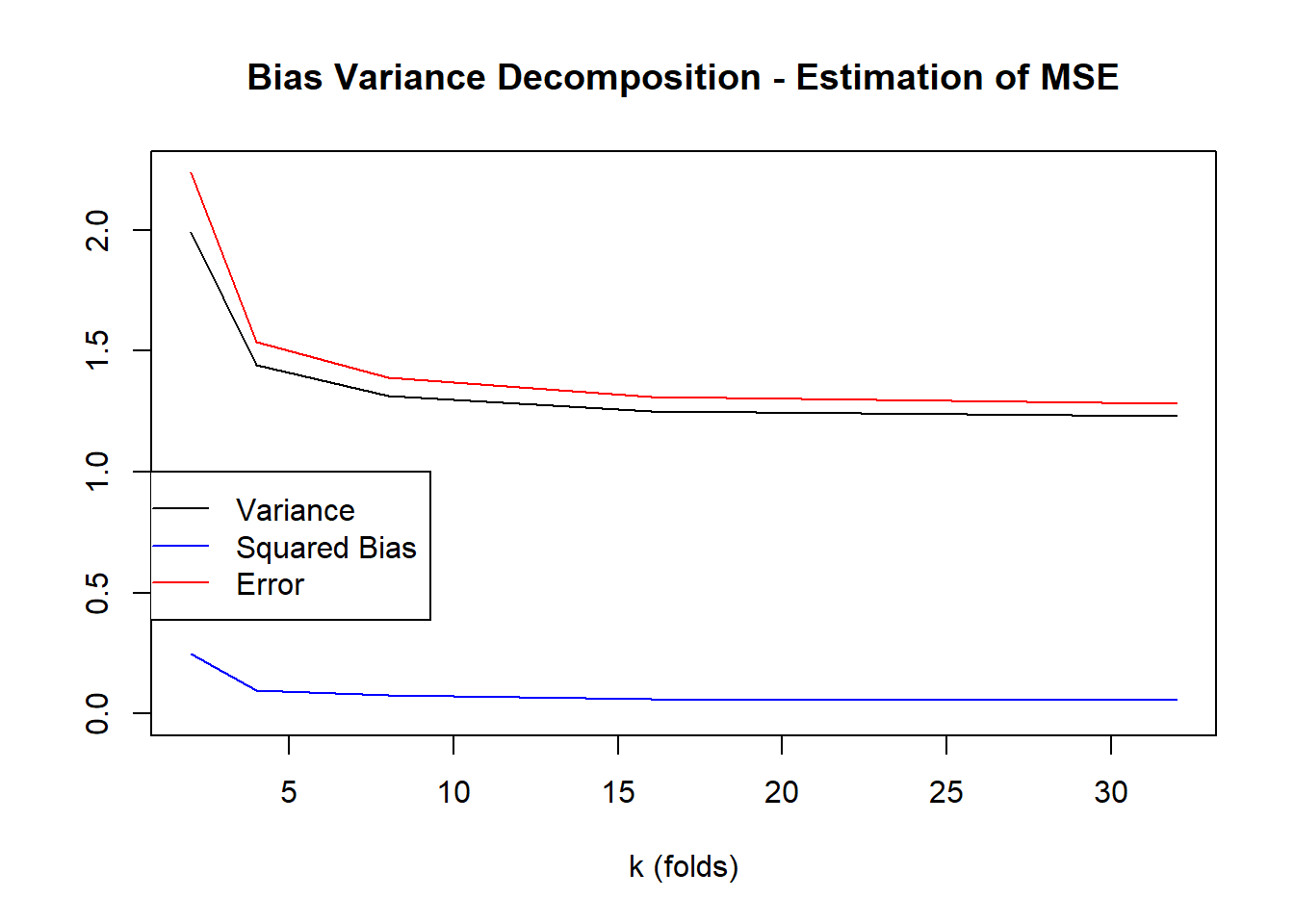
plot(trainingError~k, data=crossValidationResults, type="l", ylim=c(3,4.6))
lines(testingError~k, data=crossValidationResults, col="blue")
abline(h=2^2, col="red")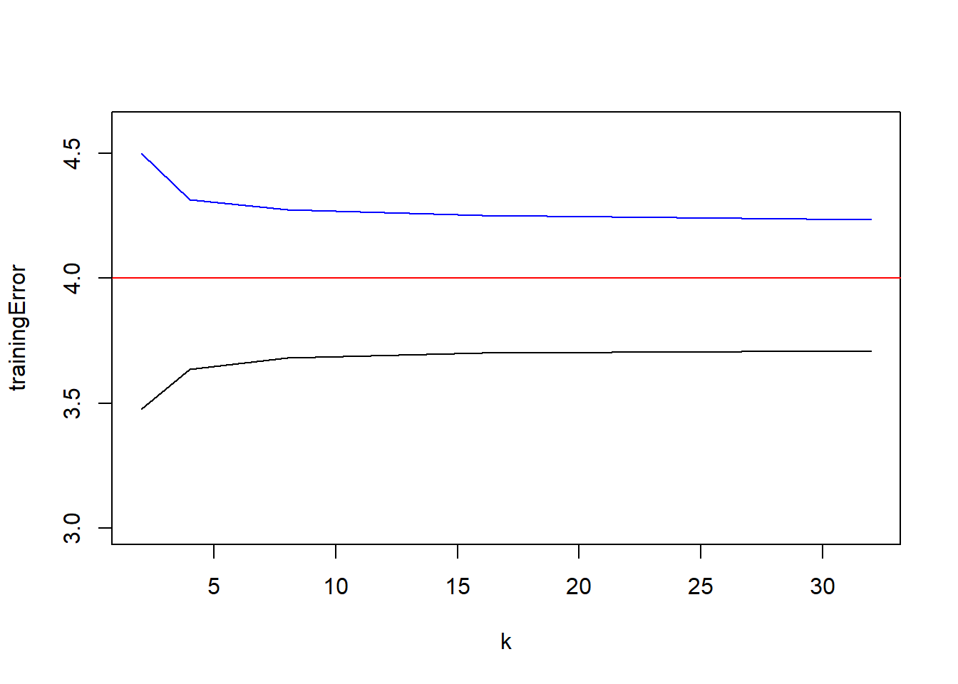
36.2 Another Example - A Multiple Regression Model
We will sample from a population, fit a linear model, then predict 1000 data points. We will actually repeat this over and over and in the end we will have 1000 model fits and for each one we will have 1000 predictions.
The true model is
\[Y_i = 10 + 2X_{1,i} + 5X_{2,i} -3X_{3,i} + \epsilon_i, \text{ where }\epsilon\sim N(0,2^2)\] This model fitting will be based on a larger sample, a sample of size 128.
generate_data <- function(n){
  X1 <- rnorm(n, 5, 4)
  X2 <- rnorm(n, 1, 4)
  X3 <- rnorm(n, 3, 4)
  eps <- rnorm(n, 0, 2)
  Y <- 10 + 2*X1 +5*X2 -3*X3+ eps
  return(data.frame(X1,X2,X3,Y))
}

NMC <- 1000
nOut <- 1000
outData <- generate_data(nOut)
n <- 128

results <- data.frame('rep' = rep(1:NMC, nOut),
                      'i' = rep(1:nOut, each=NMC),
                      'Y' = rep(outData$Y, each=NMC),
                      'Yhat' = rep(0,nOut*NMC),
                      'error'= rep(0,nOut*NMC))

for(k in 1:NMC){
  sampleData <- generate_data(128)
  modelFit <- lm(Y~., data=sampleData)
  yhat <- predict(modelFit, newdata=outData)
  results[results$rep==k,"Yhat"] <- yhat
}
results$error = results$Y-results$Yhat


predVar <- mean(aggregate(Yhat~rep, results, FUN="var")$Yhat)
predBias2 <- mean(aggregate(error~i, results, FUN="mean")$error)^2
predErr <- mean(results$error^2)

print(paste("Variance =",predVar))
[1] "Variance = 580.633211183573"print(paste("Squared Bias = ", predBias2))[1] "Squared Bias = 0.00160131358719143"print(paste("Mean Square Error = ",predErr))[1] "Mean Square Error = 4.36704941289589"print(paste("Var + Bias^2 = ",predVar+predBias2))[1] "Var + Bias^2 = 580.634812497161"print(paste("estimate of sigma = ",sqrt(predErr)))[1] "estimate of sigma = 2.08974864825794"Now we will estimate the testing errror and training error for various numbers of folds
NMC <- 250
ks <- c(2,4,8,16,32,64,128)
crossValidationResults <- data.frame('k' = ks,
trainingError = 0,
testingError = 0,
testingVariance = 0,
testingBias2 = 0,
estimationError=0)
for(K in ks){
trnErr <- 0
tstErr <- 0
for(j in 1:NMC){
set.seed(j) #same data, repeated once for each k
sampleData <- generate_data(n)
#idx is a shuffled vector of row numbers
idx <- sample(1:nrow(sampleData))
#folds partitions the row indices
folds <- split(idx, as.factor(1:K))
trainingErrors <- 0
testingErrors <- 0
for(k in 1:K){
training <- sampleData[-folds[[k]],]
testing <- sampleData[folds[[k]],]
#estimate MSE
#fit the model to the training data
modelFit <- lm(Y~., data=training)
#calculate the average squared error on the testing data
trainingErrors[k] <- mean(resid(modelFit)^2)
testingErrors[k] <- mean((predict(modelFit, newdata=testing) - testing$Y)^2)
}
trnErr[j] <- mean(trainingErrors)
tstErr[j] <- mean(testingErrors)
}
crossValidationResults[crossValidationResults$k==K, "trainingError"] <- mean(trnErr)
crossValidationResults[crossValidationResults$k==K, "testingError"] <- mean(tstErr)
crossValidationResults[crossValidationResults$k==K, "testingVariance"] <- var(tstErr)
crossValidationResults[crossValidationResults$k==K, "testingBias2"] <- mean((tstErr-4))^2
crossValidationResults[crossValidationResults$k==K, "estimationError"] <- mean((tstErr-4)^2)
}
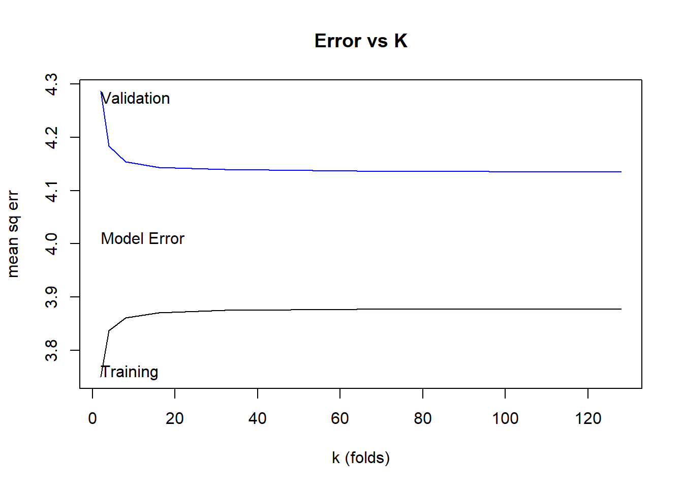
crossValidationResults k trainingError testingError testingVariance testingBias2 estimationError
1 2 3.750027 4.286584 0.4030953 0.08213047 0.4836134
2 4 3.836878 4.183352 0.3323707 0.03361782 0.3646590
3 8 3.861163 4.154025 0.3210524 0.02372356 0.3434918
4 16 3.870692 4.144120 0.3167117 0.02077066 0.3362155
5 32 3.875014 4.139478 0.3156883 0.01945414 0.3338797
6 64 3.877074 4.137198 0.3139791 0.01882324 0.3315464
7 128 3.878085 4.134802 0.3129656 0.01817168 0.3298854plot(testingVariance~k, data=crossValidationResults, type="l", main="Bias Variance Decomposition - Estimation of MSE", ylim=c(0, max(crossValidationResults$estimationError)), ylab="", xlab="k (folds)")
lines(testingBias2~k, data=crossValidationResults, col="blue")
lines(estimationError~k, data=crossValidationResults, col="red")
legend(0,1,legend=c("Variance","Squared Bias","Error"), col=c("black","blue","red"), lty=1)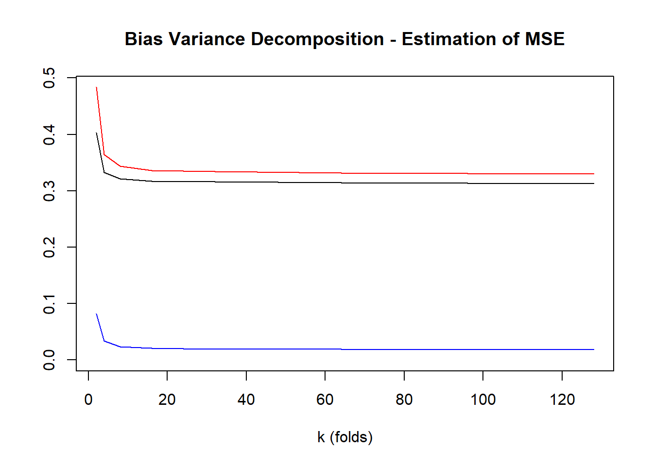
plot(trainingError~k, data=crossValidationResults, type="l", ylim=range(crossValidationResults[,2:3]), main="Error vs K", ylab="mean sq err",xlab="k (folds)")
lines(testingError~k, data=crossValidationResults, col="blue")
abline(h=predErr, col="red")
text(2, crossValidationResults$testingError[1],"Validation",adj=c(0,1))
text(2, crossValidationResults$trainingError[1],"Training",adj=c(0,0))
text(2, 4,"Model Error",adj=c(0,0))