The farmer selects 5 of her calves and divides them into two groups. One group contains 2, the other group has 3 animals. The first group she protects using impregnated ear tags. To the other group she applies an oil-based formulation of the same insecticide, an artificial pyrethroid. The farmer pens each calf separately, and estimates the number of stable-flies in each pen by hanging sticky flypaper above the animal. After 3 days she removes her flypapers and counts the number of stable-flies on each.
Flypaper number
1
2
3
4
5
Flies caught
30
50
7
12
30
Treatment
tag
tag
pour
pour
pour
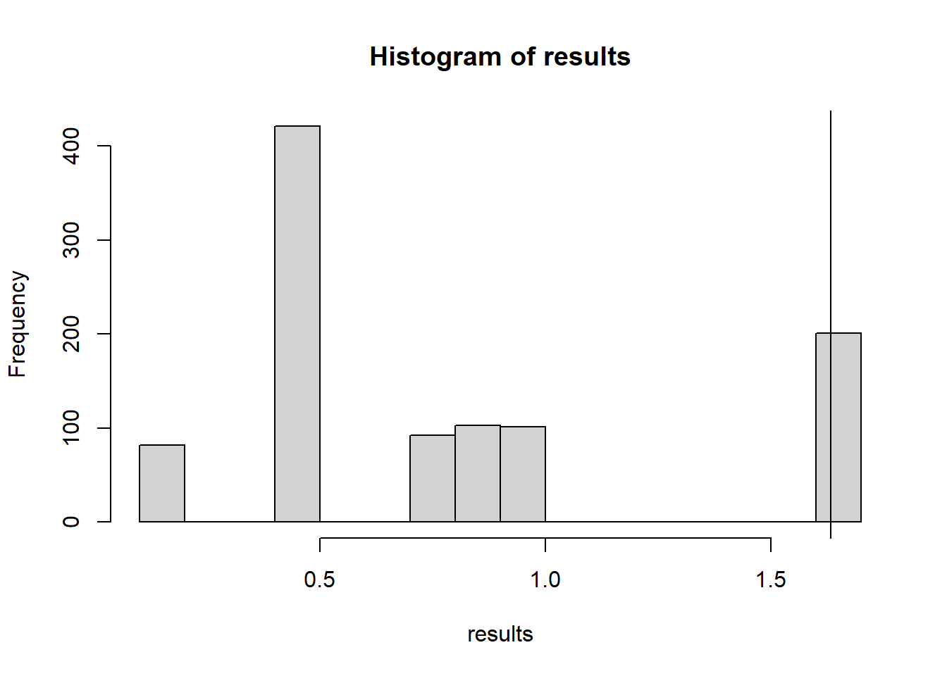
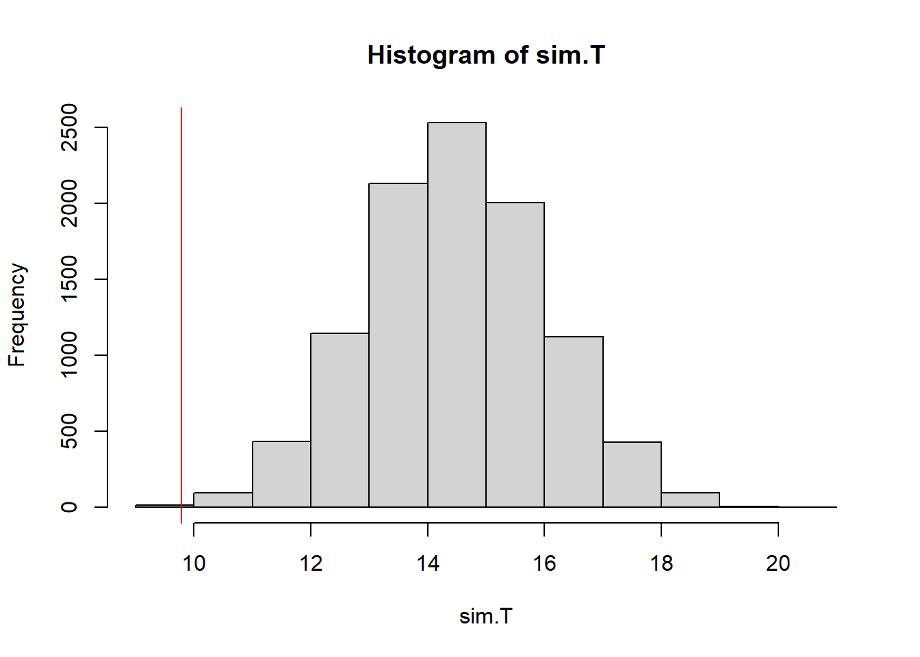
Use the ratio of flies caught as a test statistic. How strong is the evidence that the pour-on treatment is more effective at repelling flies. (lower number of flies caught means flies are repelled)
The probability that we observe a test statistic as extreme as we observed is 0.201, which means that the observed data would not be unusual if the treatment did not have differing effects. In other words, if the number of flies on each of the cows was drawn from the same population (regardless of treatment) we’d observe data like we had about 20% of the time, which is not very low, so we would not reject the null hypothesis.
16.2 Babies
We will use the following dataset to demonstrate the use of permutations:
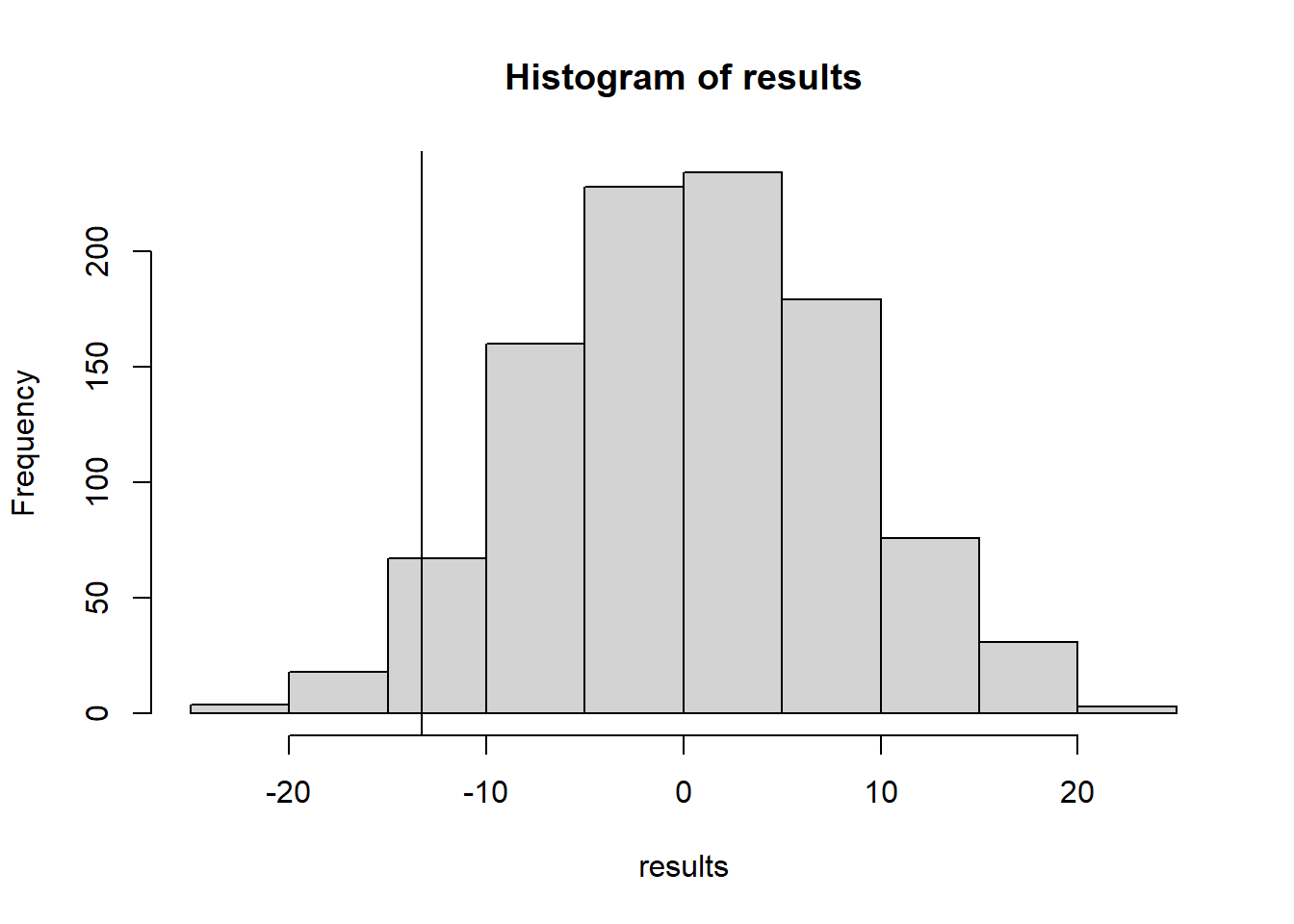
The question is whether this observed difference is statistically significant. We do not want to rely on the assumptions needed for the normal or t-distribution approximations to hold, so instead we will use permutations.
The null hypothesis is that the distribution of birthweights for smokers is the same as the distribution for nonsmokers. The alternative hypothesis is that the mean birthweight for smokers is lower than for nonsmokers.
The observed test statistic has a p-value of 0.042; If the distributions are the same, we would only observe a difference of sample means this (or more) extreme 4.2% of the time, and this is lower than our significance level of 0.05, so we have strong evidence against the null hypothesis. There’s strong evidence that the mean birthweight is lower for smokers.
16.3 Best age?
If you could stop time and live forever in good health at a particular age, at what age would you like to live?”
Suppose we are interested in testing the claim that the average ideal age for women is greater than men. A random sample of 3 women and 3 men were asked this question resulting in the following responses:
The permutation test does not provide us evidence to support the claim; We lack evidence that the mean ideal age for women is greater than the mean ideal age for men.
Suppose that you work at a bicycle factory where you’d like to replace steel tubes in the company’s bicycle frames with titanium (because it’s lighter). You have carefully selected random samples of the steel and titanium tubes from your suppliers. You measure the stiffness of each tube in a testing rig. The data are (measured in pounds per square inch, psi):
Steel: 30.7, 29.5, 29.8, 30.3, 29.2
Titanium: 29.9, 31.1, 30.2, 30.8, 30.7, 31.9
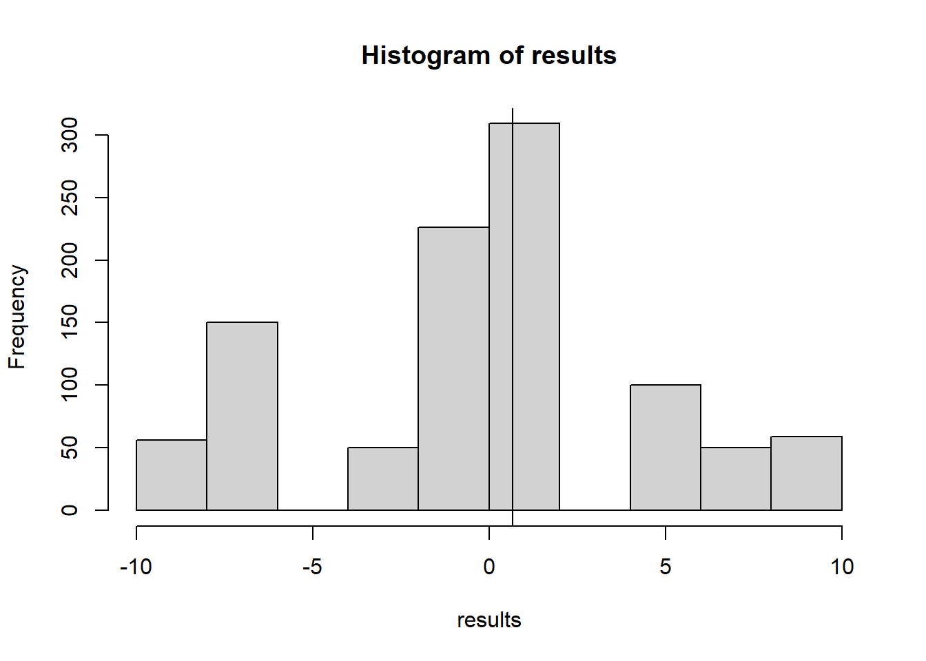
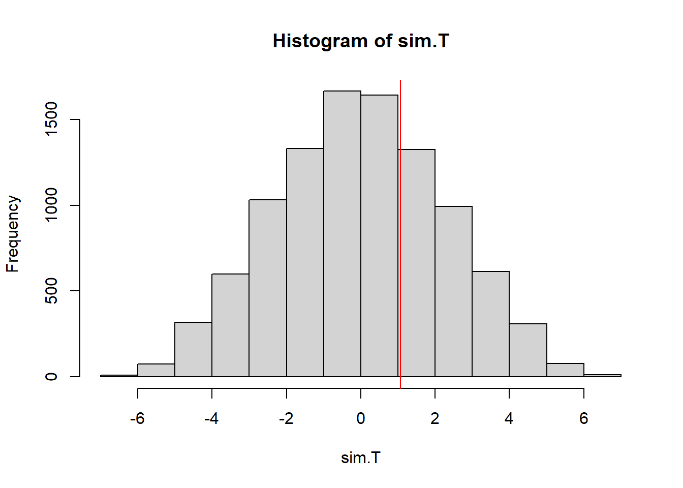
Perform a permutation test to see if there is evidence that the mean stiffness is different between steel and titanium. Use the difference of sample means as a test statistic and perform a two-tailed test.
Our 2-tailed p-value is 0.046, which is lower than our significance threshold of 0.05; we have good evidence that the mean stiffness of titanium frames is different than the mean stiffness of steel frames.
16.4 Maximum Current
(From Introduction to Probability and Statistics for Data Science)
An electrical engineer must design a circuit to deliver the maximum amount of current to a display tube to achieve sufficient image brightness. Within her allowable design constraints, she has developed two candidate circuits and tests prototypes of each. The resutling data (in microamperes) are
Circuit 1: 251, 255, 258, 257, 250, 251, 254, 250
Circuit 2: 250, 253, 249, 256, 259, 252, 260, 251
Develop and test an appropriate hypothesis for this problem using Monte Carlo
Repeat the test but this time use an appropriate parametric test. What assumptions are made?
16.5 Rank-based permutation test
Researchers compared the effectiveness of conventional textbook worked examples to modified worked examples, which present the algebraic manipulations and explanation as part of the graphical display. They are interested if the time to complete problems improves if students can study from the modified examples compared to the conventional examples.
Subjects: 28 ninth-year students in Sydney, Australia, with no previous exposure to coordinate geometry but have adequate math to deal with the problems given The 28 subjects were randomized to self-study one of two instructional materials. The two materials covered exactly the same problems, presented differently. Students were given as much time as they wished to study the material, but not allowed to ask questions. Following the instructional phase, all students were tested with a common examination over three problems of different difficulty. Response: the time (in seconds) required to arrive at a solution to the moderately difficult problem.
Note the response is censored at 300 seconds because the time allotment for the problem is 5 minutes Five students did not complete the problem in the 5-minute (300 seconds) time allotment.
Solution
Because of the data truncated at 300, it’s reasonable to convert the values to ranks. This will also handle strangeness in distribution shape. We could use any statistic based on rank as a test statistic. We’ll use the mean rank from the modified group. Difference of means would be equivalent - it wouldn’t be a more powerful test statistic (you can verify this).
We would find evidence for the claim if the mean rank from the modified group is particularly low, so this is a left-sided test.
The \(p\)-value is extremely low, we have overwhelming evidence that the modified problems tend to result in lower completion time
16.6 Paired sample permutation test
Two body designs are being considered for a new car model. The time (in seconds) to parallel park each body design was recorded for 14 drivers. The following results were obtained.
Driver
1
2
3
4
5
6
7
8
9
10
11
12
13
14
Model 1
37.0
25.8
16.2
24.2
22.0
33.4
23.8
43.2
33.6
24.4
23.4
21.2
36.2
32.8
Model 2
17.8
20.2
16.8
41.4
21.4
38.4
16.8
34.2
27.8
23.2
29.6
20.6
32.2
41.8
Does this data give us strong evidence that the mean time to parallel park is different for the two body designs? Use a Monte Carlo test
Solution
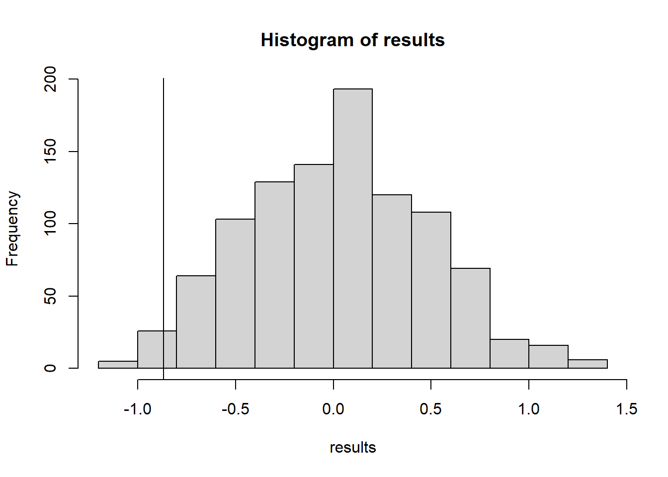
The null hypothesis is that each pair of values are equally likely to be for Model 1/ Model 2 as it would be for Model 2/Model 1. The permutation thus would not be across drivers, but across models.
The \(p\)-value is above .65; If the null hypothesis were true, and the two times were just due to driver and had nothing to do with the model, we’d see a test statistic this extreme (or more) 65% of the time.
17 Beyond STAT 340
These problems are excellent practice but they are beyond the material we cover in STAT 340.