85+ 10*4 + .07*110 + 0.01*4*110[1] 137.1Suppose we have a data set with five predictors, \(X_1 =\) GPA, \(X_2 =\) IQ, $X_3 =$ Level ( \(1\) for College and \(0\) for High School), \(X_4\) = Interaction between GPA and IQ, and \(X_5\) = Interaction between GPA and Level. The response is starting salary after graduation (in thousands of dollars). Suppose we use least squares to fit the model, and get \(\hat{\beta}_0=50, \hat{\beta}_1=20, \hat{\beta}_2=0.07, \hat{\beta}_3=35, \hat{\beta}_4=0.01\) and \(\hat{\beta}_5 = -10\).
Which answer is correct, and why?
For a fixed value of IQ and GPA, high school graduates earn more, on average, than college graduates.
For a fixed value of IQ and GPA, college graduates earn more, on average, than high school graduates.
For a fixed value of IQ and GPA, high school graduates earn more, on average, than college graduates provided that the GPA is high enough.
For a fixed value of IQ and GPA, college graduates earn more, on average, than high school graduates provided that the GPA is high enough.
It helps to write out the estimated model with variable names:
\[\widehat{Salary} = 50 + 20(GPA)+0.07(IQ) + 35(1_{college})+0.01(GPA \times IQ) -10 (GPA \times 1_{college})\]
If we fix IQ and GPA, the models for salaries are:
\[\widehat{Salary}_{HS} = 50 + 20(GPA)+0.07(IQ) +0.01(GPA \times IQ)\]
\[\widehat{Salary}_{C} = 85 + 10(GPA)+0.07(IQ) +0.01(GPA \times IQ)\]
If we compare these two you can see that the effect of higher GPA is more substantial for high school students. What is the difference in salary?
\[ \widehat{Salary}_{C}-\widehat{Salary}_{HS} = 35-10(GPA)\] If \(GPA < 3.5\) this difference is positive (i.e. college grads earn a higher salary). If \(GPA > 3.5\) then the difference is negative (i.e. high school grads earn higher salary)
Thus iii is the correct choice.
85+ 10*4 + .07*110 + 0.01*4*110[1] 137.1The predicted salary is $137.1
The magnitude of the coefficient has nothing to do with the level of evidence of the interaction. It’s all relative to the standard error of this coefficient. A small magnitude coefficient with a very small standard error would have very little uncertainty. If the standard error is big that would mean the uncertainty is great. This is why we take the ratio of \(\hat{\beta}_j/se(\hat{\beta}_j)\)
I collect a set of data ($n = 100$ observations) containing a single predictor and a quantitative response. I then fit a linear regression model to the data, as well as a separate cubic regression, i.e. \(Y = \beta_0 + \beta_1X + \beta_2X^2 + \beta_3X^3 + \epsilon\).
In expectation (in the sense of expected value) we would expect \(\hat{\beta}_2=\hat{\beta}_3=0\) and then RSS would be the same for both the linear and the cubic model. However in practice the data will not exhibit a perfect straight line relationship and thus these coefficients will be nonzero. That would mean the cubic model will fit slightly better and RSS will be lower for the cubic model.
A cubic model would presumably slightly overfit to the training data, and could actually perform worse on test data, data that is drawn from a truly linear model. So we would expect test RSS to be lower with the cubic model.
Without knowing what the relationship is, this would be hard to answer. However if there is any curve to the true relationship a cubic model will most likely fit the training data better and will give us a lower RSS than a linear model.
This question involves the use of simple linear regression on the Auto data set.
lm() function to perform a simple linear regression with mpg as the response and horsepower as the predictor. Use the summary() function to print the results. Comment on the output.For example:
i. Is there a relationship between the predictor and the response?
ii. How strong is the relationship between the predictor and the response?
iii. Is the relationship between the predictor and the response positive or negative?
iv. What is the predicted mpg associated with a horsepower of 98? What are the associated 95% confidence and prediction intervals?
library(ISLR)Warning: package 'ISLR' was built under R version 4.2.3auto.fit <- lm(mpg~1+horsepower, data=Auto)
summary(auto.fit)
Call:
lm(formula = mpg ~ 1 + horsepower, data = Auto)

Residuals:
     Min       1Q   Median       3Q      Max
-13.5710  -3.2592  -0.3435   2.7630  16.9240

Coefficients:
             Estimate Std. Error t value Pr(>|t|)
(Intercept) 39.935861   0.717499   55.66   <2e-16 ***
horsepower  -0.157845   0.006446  -24.49   <2e-16 ***
---
Signif. codes:  0 '***' 0.001 '**' 0.01 '*' 0.05 '.' 0.1 ' ' 1

Residual standard error: 4.906 on 390 degrees of freedom
Multiple R-squared:  0.6059,    Adjusted R-squared:  0.6049
F-statistic: 599.7 on 1 and 390 DF,  p-value: < 2.2e-16
There is a very strong relationship between the predictor and response. The p-value is close to zero meaning this data would be virtually impossible if the relationship was not real. The relationship is negative, clearly by the sign of the coefficient. Higher horsepower vehicles tend on average to have lower fuel efficiency.
predict(auto.fit, newdata=data.frame(horsepower=98), interval="confidence") fit lwr upr
1 24.46708 23.97308 24.96108predict(auto.fit, newdata=data.frame(horsepower=98), interval="prediction") fit lwr upr
1 24.46708 14.8094 34.12476A vehicle with 98 horsepower has a predicted fuel efficiency of 24.47 mpg. The 95% confidence interval says that we are 95% confident that the average mpg of cars with 98 horsepower is within 23.97 and 24.96 mpg. The 95% prediction interval tells us that if we pick one arbitrary car with a horsepower of 98, we are 95% confident that its mpg will be within 13.81 and 34.12 mpg. You can tell that there is quite a bit of variation among cars.
Plot the response and the predictor. Use the abline() function to display the least squares regression line.
Use the plot() function to produce diagnostic plots of the least squares regression fit. Comment on any problems you see with the fit.
This question involves the use of multiple linear regression on the Auto data set.
Produce a scatterplot matrix which includes all of the variables in the data set.
Compute the matrix of correlations between the variables using the function cor(). You will need to exclude the name variable, cor() which is qualitative.
Use the lm() function to perform a multiple linear regression with mpg as the response and all other variables except name as the predictors. Use the summary() function to print the results. Comment on the output. For instance:
i. Is there a relationship between the predictors and the response?
ii. Which predictors appear to have a statistically significant relationship to the response?
iii. What does the coefficient for the year variable suggest?
Use the plot() function to produce diagnostic plots of the linear regression fit. Comment on any problems you see with the fit. Do the residual plots suggest any unusually large outliers? Does the leverage plot identify any observations with unusually high leverage?
Use the * and : symbols to fit linear regression models with interaction effects. Do any interactions appear to be statistically significant?
Try a few different transformations of the variables, such as \(log(X)\), \(\sqrt{X}\), \(X^2\). Comment on your findings.
This question should be answered using the Carseats data set.
Fit a multiple regression model to predict Sales using Price, Urban, and US.
Provide an interpretation of each coefficient in the model. Be careful—some of the variables in the model are qualitative!
Write out the model in equation form, being careful to handle the qualitative variables properly.
For which of the predictors can you reject the null hypothesis \(H_0 : \beta_j = 0\)?
On the basis of your response to the previous question, fit a smaller model that only uses the predictors for which there is evidence of association with the outcome.
How well do the models in (a) and (e) fit the data?
Using the model from (e), obtain 95% confidence intervals for the coefficient(s).
Is there evidence of outliers or high leverage observations in the model from (e)?
In this exercise you will create some simulated data and will fit simple linear regression models to it. Make sure to use set.seed(1) prior to starting part (a) to ensure consistent results.
Using the rnorm() function, create a vector, x, containing \(100\) observations drawn from a \(N(0, 1)\) distribution. This represents a feature, \(X\).
Using the rnorm() function, create a vector, eps, containing \(100\) observations drawn from a \(N(0, 0.5^2)\) distribution—a normal distribution with mean zero and variance 0.25.
Using x and eps, generate a vector y according to the model \(Y = −1 + 0.5X + \epsilon\). What is the length of the vector y? What are the values of \(\beta_0\) and \(\beta_1\) in this linear model?
Create a scatterplot displaying the relationship between x and y. Comment on what you observe.
Fit a least squares linear model to predict y using x. Comment on the model obtained. How do \(\hat{\beta}_0\) and \(\hat{\beta}_1\) compare to \(\beta_0\) and \(\beta_1\)?
Display the least squares line on the scatterplot obtained in (d). Draw the population regression line on the plot, in a different color. Use the legend() command to create an appropriate legend.
Now fit a polynomial regression model that predicts y using x and x^2. Is there evidence that the quadratic term improves the model fit? Explain your answer.
Repeat (a)–(f) after modifying the data generation process in such a way that there is less noise in the data. The model should remain the same. You can do this by decreasing the variance of the normal distribution used to generate the error term \(\epsilon\) in (b). Describe your results.
Repeat (a)–(f) after modifying the data generation process in such a way that there is more noise in the data. The model should remain the same. You can do this by increasing the variance of the normal distribution used to generate the error term in (b). Describe your results.
What are the confidence intervals for \(\beta_0\) and \(\beta_1\) based on the original data set, the noisier data set, and the less noisy data set? Comment on your results.
This problem focuses on the collinearity problem.
set.seed (1)
x1 <- runif(100)
x2 <- 0.5 * x1 + rnorm(100) / 10
y <- 2 + 2 * x1 + 0.3 * x2 + rnorm(100)
The last line corresponds to creating a linear model in which y is a function of x1 and x2. Write out the form of the linear model. What are the regression coefficients?
What is the correlation between x1 and x2? Create a scatterplot displaying the relationship between the variables.
Using this data, fit a least squares regression to predict y using x1 and x2. Describe the results obtained. What are \(\hat{\beta}_0\), \(\hat{\beta}_1\) and \(\hat{\beta}_2\)? How do these relate to the true \(\beta_0\), \(\beta_1\), and \(\beta_2\)? Can you reject the null hypothesis \(H_0 : \beta_1 = 0\)? How about the null hypothesis \(H_0 : \beta_2 = 0\)?
Now fit a least squares regression to predict y using only x1. Comment on your results. Can you reject the null hypothesis \(H_0 : \beta_1 = 0\)?
Now fit a least squares regression to predict y using only x2. Comment on your results. Can you reject the null hypothesis \(H_0 : \beta_1 = 0\)?
Do the results obtained in (c)–(e) contradict each other? Explain your answer.
Now suppose we obtain one additional observation, which was unfortunately mismeasured.
x1 <- c(x1 , 0.1)
x2 <- c(x2 , 0.8)
y <- c(y, 6)
Re-fit the linear models from (c) to (e) using this new data. What effect does this new observation have on the each of the models? In each model, is this observation an outlier? A high-leverage point? Both? Explain your answers.
This problem involves the Boston data set. We will now try to predict per capita crime rate using the other variables in this data set. In other words, per capita crime rate is the response, and the other variables are the predictors.
For each predictor, fit a simple linear regression model to predict the response. Describe your results. In which of the models is there a statistically significant association between the predictor and the response? Create some plots to back up your assertions.
Fit a multiple regression model to predict the response using all of the predictors. Describe your results. For which predictors can we reject the null hypothesis \(H_0 : \beta_j = 0\)?
How do your results from (a) compare to your results from (b)? Create a plot displaying the univariate regression coefficients from (a) on the \(x\)-axis, and the multiple regression coefficients from (b) on the \(y\)-axis. That is, each predictor is displayed as a single point in the plot. Its coefficient in a simple linear regression model is shown on the \(x\)-axis, and its coefficient estimate in the multiple linear regression model is shown on the \(y\)-axis.
Is there evidence of non-linear association between any of the predictors and the response? To answer this question, for each predictor X, fit a model of the form
\(Y = \beta_0 + \beta_1X + \beta_2X^2 + \beta_3X^3 + \epsilon.\)
The rock data set, which comes packaged with R, describes 48 rock samples taken at a petroleum reservoir. Each sample has four measurements, all related to measuring permeability of the rock (the geological details are not so important, here):
area: the area of the pores (measured in a number of pixels out of a 256-by-256 image that were “pores”)peri: perimeter of the “pores” part of the sampleshape: perimeter(peri) of the pores part divided by square root of the area (area)perm: a measurement of permeability (in milli-Darcies, a unit of permeability, naturally)Suppose that our goal is to predict permeability (perm) from other characteristics of the rock.
For each of the three other variables area, peri and shape, fit a linear regression model that predicts perm from this variable and an intercept term. That is, you should fit three models, each using one of area, peri and shape.
area_lm <- lm(perm ~ 1 + area, data=rock)
peri_lm <- lm(perm ~ 1 + peri, data=rock)
shape_lm <- lm(perm ~ 1 + shape, data=rock)
Part b: comparing fits
Compute the RSS for each of the three models fitted in Part a. Which is best?
my_rss <- function( fitted_model ) {
  return( sum( (fitted_model$residuals)**2 ) )
}
mapply( my_rss, list(area_lm, peri_lm, shape_lm) )
[1] 7591852 4092864 6216896The model using peri to predict perm achieves the smallest RSS.
Part c: multiple regression
Now, fit a model that predicts perm from the other three variables (you should not include any interaction terms).
# TODO: replace NA with model-fitting code
full_lm <- lm( perm ~ 1 + area + peri + shape, data=rock )

summary(full_lm)
Call:
lm(formula = perm ~ 1 + area + peri + shape, data = rock)

Residuals:
    Min      1Q  Median      3Q     Max
-750.26  -59.57   10.66  100.25  620.91

Coefficients:
             Estimate Std. Error t value Pr(>|t|)
(Intercept) 485.61797  158.40826   3.066 0.003705 **
area          0.09133    0.02499   3.654 0.000684 ***
peri         -0.34402    0.05111  -6.731 2.84e-08 ***
shape       899.06926  506.95098   1.773 0.083070 .
---
Signif. codes:  0 '***' 0.001 '**' 0.01 '*' 0.05 '.' 0.1 ' ' 1

Residual standard error: 246 on 44 degrees of freedom
Multiple R-squared:  0.7044,    Adjusted R-squared:  0.6843
F-statistic: 34.95 on 3 and 44 DF,  p-value: 1.033e-11
Part d: interpreting model fits
Consider the coefficient of peri in the model from Part c.
The estimated coefficient of peri is statistically significantly different from zero at the \(0.01\) level (the p-value is approximately \(3*10^{-8}\)).
The estimate of the coefficient indicates that holding area and shape constant, a unit increase in peri is associated with a decrease of \(0.344\) in perm.
The trees data set in R contains measurements of diameter (in inches), height (in feet) and the amount of timber (volume, in cubic feet) in each of 31 trees. See ?trees for additional information.
The code below loads the data set. Note that the column of the data set encoding tree diameter is mistakenly labeled Girth (girth is technically a measure of circumference, not a diameter).
data(trees)
head(trees)
Girth Height Volume
1 8.3 70 10.3
2 8.6 65 10.3
3 8.8 63 10.2
4 10.5 72 16.4
5 10.7 81 18.8
6 10.8 83 19.7Part a: examining correlations
It stands to reason that the volume of timber in a tree should scale with both the height of the tree and the diameter. However, it also stands to reason that height and diameter are highly correlated. Use the cor function to compute the pairwise correlations among the three variables.
cor(trees) Girth Height Volume
Girth 1.0000000 0.5192801 0.9671194
Height 0.5192801 1.0000000 0.5982497
Volume 0.9671194 0.5982497 1.0000000Suppose that we had to choose either tree diameter (labeled Girth in the data) or tree height with which to predict volume. Based on these correlations, Which would you choose? Why?
Girth has a much higher correlation with Volume than does Height, so it is likely to be a better predictor.
Part b: comparing model fits
Well, let’s put the above to a test. Use lm to fit two linear regression models from this data set (both should, of course, include intercept terms):
Girth in the data set)ht_lm <- lm( Volume ~ 1 + Height, data=trees );
gr_lm <- lm( Volume ~ 1 + Girth, data=trees );
c( my_rss(ht_lm), my_rss(gr_lm) )[1] 5204.8950 524.3025Compare the sum of squared residuals of these two models. Which is better? Does this agree with your observations in Part a?
The model predicting volume from girth is indeed a better model, achieving a factor of ten decrease in RSS compared to the model using height. This is in agreement with the prediction in part a.
Examining the model outputs above (or extracting information again here), what do each of your fitted models conclude about the null hypothesis that the slope is equal to zero?
summary( ht_lm )
Call:
lm(formula = Volume ~ 1 + Height, data = trees)

Residuals:
    Min      1Q  Median      3Q     Max
-21.274  -9.894  -2.894  12.068  29.852

Coefficients:
            Estimate Std. Error t value Pr(>|t|)
(Intercept) -87.1236    29.2731  -2.976 0.005835 **
Height        1.5433     0.3839   4.021 0.000378 ***
---
Signif. codes:  0 '***' 0.001 '**' 0.01 '*' 0.05 '.' 0.1 ' ' 1

Residual standard error: 13.4 on 29 degrees of freedom
Multiple R-squared:  0.3579,    Adjusted R-squared:  0.3358
F-statistic: 16.16 on 1 and 29 DF, p-value: 0.0003784summary( gr_lm )
Call:
lm(formula = Volume ~ 1 + Girth, data = trees)

Residuals:
   Min     1Q Median     3Q    Max
-8.065 -3.107  0.152  3.495  9.587

Coefficients:
            Estimate Std. Error t value Pr(>|t|)
(Intercept) -36.9435     3.3651  -10.98 7.62e-12 ***
Girth         5.0659     0.2474   20.48  < 2e-16 ***
---
Signif. codes:  0 '***' 0.001 '**' 0.01 '*' 0.05 '.' 0.1 ' ' 1

Residual standard error: 4.252 on 29 degrees of freedom
Multiple R-squared:  0.9353,    Adjusted R-squared:  0.9331
F-statistic: 419.4 on 1 and 29 DF,  p-value: < 2.2e-16
Both models conclude that the coefficient of the single predictor is statistically significantly different from zero at level \(0.001\).
Part c: volume and diameter
Thinking back to fourth grade geometry with Mrs. Galvin, you remember that the area of a circle grows like the square of the diameter (that is, if we double the diameter, the area of the circle quadruples). It follows that timber volume, which is basically the volume of a cylinder, should scale linearly with the square of the diameter.
Create a scatter plot of volume as a function of diameter. Does the “geometric” intuition sketched above agree with what you see in the plot? Why or why not?
plot(trees$Girth, trees$Volume)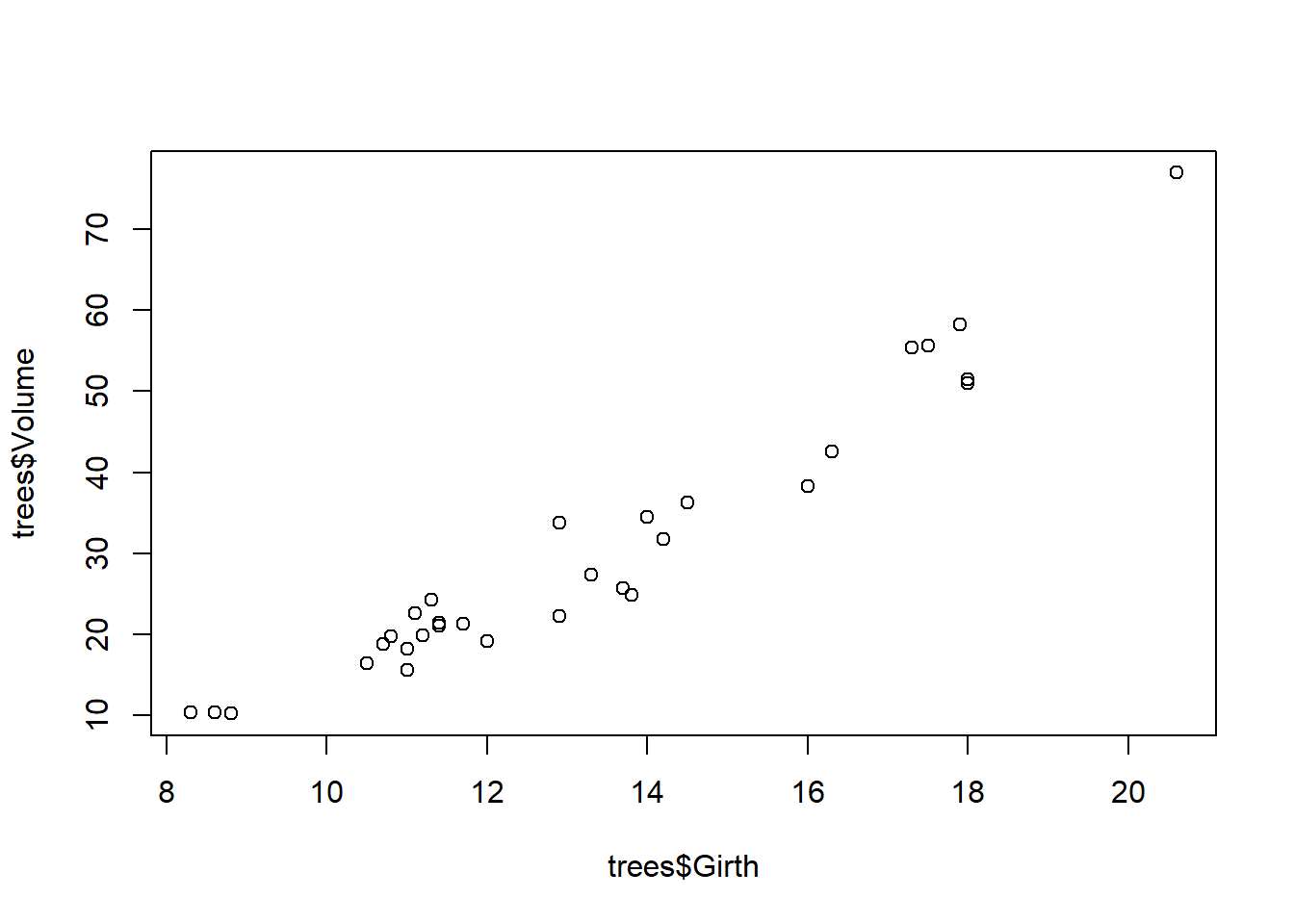
At least visually, this looks like a simple linear relationship. It doesn’t appear that using squared diameter should change anything in terms of prediction performance.
Part d: incorporating non-linearities
Fit a linear regression model predicting volume from the squared diameter (and an intercept term, of course). Compute the residual sum of squares of this model.
diam2_lm <- lm( Volume ~ 1 + I(Girth^2), data=trees)

my_rss( diam2_lm )
[1] 329.3191Compare the RSS of this model with that obtained in Part b using the linear diameter. Which is better, the quadratic model or the linear model? Does this surprise you? Why or why not? If you are surprised, what might explain the observation?
This is indeed notably smaller than the RSS achieved by the linear model. This is surprising given that there is no clear nonlinearity in the scatterplot, but it is in keeping with our “geometric” intuition.
These problems are excellent practice but they are beyond the material we cover in STAT 340.