5  Probability and Random Variables Practice

6 Practice Problems

6.1 Phone Repair

(From Introduction to Probability and Statistics for Data Science) The repair of a broken cell phone is either completed on time or it is late and the repair is either done satisfactorily or unsatisfactorily. What is the sample space for a cell phone repair?

Solution

The sample space consists of two outcomes: {satisfactory, unsatisfactory}

6.2 Dice Probabilities I

What is the probability that at least one of the following events occurs on a single throw of two fair six-sided dice?

1. The dice total 5.

2. The dice total 6.

3. The dice total 7.

Solution

The probability that at least one of the following occurs requires us to look at the union of the events. “The dice total is 5, 6 or 7”.

On a single throw of two fair dice, the dice total can be a single number, so events A, B and C are mutually exclusive. We can calculate the probabilities individually and add them up.

A 5 can occur in 4 ways: \((1,4), (2,3), (3,2), (4,1)\) are the four ways (we are distinguishinng the two dice).

A 6 can occur in 5 ways: \((1,5), (2,4), (3,3), (4,2), (5,1)\).

A 7 can occur in 6 ways: \((1,6), (2,5), (3,4), (4,3), (5,2), (6,1)\)

In the end, there are \(4+5+6 = 15\) ways in which one of these events can occur. Since there are \(6\times 6=36\) two-dice outcomes, the probability is \[\frac{15}{36}\]

6.3 Dice Probabilities II

What is the probability that at least one of the following events occurs on a single throw of two fair four-sided dice?

1. The dice total 5.

2. The dice total 6.

3. The dice total 7.

Solution

A 5 can occur in 4 ways: \((1,4), (2,3), (3,2), (4,1)\) are the four ways (we are distinguishing the two dice).

A 6 can occur in 3 ways: \((2,4), (3,3), (4,2)\).

A 7 can occur in 2 ways: \((3,4), (4,3)\)

In the end, there are \(4+3+2 = 9\) ways in which one of these events can occur. Since there are \(4\times 4=16\) two-dice outcomes, the probability is \[\frac{9}{16}\]

6.4 Two Fair Coins

Alex and Bob each flips a fair coin twice. Use “1” to denote heads and “0” to denote tails. Let X be the maximum of the two numbers Alex gets, and let Y be the minimum of the two numbers Bob gets.

1. Find and sketch the joint PMF \(p_{X,Y} (x, y)\).

2. Find the marginal PMF \(p_X(x)\) and \(p_Y (y)\).

3. Find the conditional PMF \(P_{X|Y} (x | y)\). Does \(P_{X|Y} (x | y) = P_X(x)\)? Why or why not?

Solution

x <- 0:1
px <- c(.25, .75) 

y<- 0:1
py <- c(.75, .25)

pmf <- px %*% t(py)
rownames(pmf) <- x
colnames(pmf) <- y 
addmargins(pmf)

         0      1  Sum
0   0.1875 0.0625 0.25
1   0.5625 0.1875 0.75
Sum 0.7500 0.2500 1.00

prop.table(pmf, 2)

     0    1
0 0.25 0.25
1 0.75 0.75

Each column gives P(X=x|Y=y) for the two values of y; you can see that they are the same; the reason is because the value of X and Y are independent.

6.5 Two Fair Dice

Two fair dice are rolled. Find the joint PMF of \(X\) and \(Y\) when

1. \(X\) is the larger value rolled, and \(Y\) is the sum of the two values.

Solution

die1 <- rep(1:6, 6)
die2 <- rep(1:6, rep(6,6))
outcomes <- data.frame(die1, die2)
outcomes$x <- pmax(die1, die2)
outcomes$y <- die1+die2
pmf <- prop.table(table(outcomes$x, outcomes$y))
pmf

   
             2          3          4          5          6          7
  1 0.02777778 0.00000000 0.00000000 0.00000000 0.00000000 0.00000000
  2 0.00000000 0.05555556 0.02777778 0.00000000 0.00000000 0.00000000
  3 0.00000000 0.00000000 0.05555556 0.05555556 0.02777778 0.00000000
  4 0.00000000 0.00000000 0.00000000 0.05555556 0.05555556 0.05555556
  5 0.00000000 0.00000000 0.00000000 0.00000000 0.05555556 0.05555556
  6 0.00000000 0.00000000 0.00000000 0.00000000 0.00000000 0.05555556
   
             8          9         10         11         12
  1 0.00000000 0.00000000 0.00000000 0.00000000 0.00000000
  2 0.00000000 0.00000000 0.00000000 0.00000000 0.00000000
  3 0.00000000 0.00000000 0.00000000 0.00000000 0.00000000
  4 0.02777778 0.00000000 0.00000000 0.00000000 0.00000000
  5 0.05555556 0.05555556 0.02777778 0.00000000 0.00000000
  6 0.05555556 0.05555556 0.05555556 0.05555556 0.02777778

2. \(X\) is the smaller, and \(Y\) is the larger value rolled.

Solution

die1 <- rep(1:6, 6)
die2 <- rep(1:6, rep(6,6))
outcomes <- data.frame(die1, die2)
outcomes$x <- pmin(die1, die2)
outcomes$y <- pmax(die1,die2)
pmf <- prop.table(table(outcomes$x, outcomes$y))
pmf

   
             1          2          3          4          5          6
  1 0.02777778 0.05555556 0.05555556 0.05555556 0.05555556 0.05555556
  2 0.00000000 0.02777778 0.05555556 0.05555556 0.05555556 0.05555556
  3 0.00000000 0.00000000 0.02777778 0.05555556 0.05555556 0.05555556
  4 0.00000000 0.00000000 0.00000000 0.02777778 0.05555556 0.05555556
  5 0.00000000 0.00000000 0.00000000 0.00000000 0.02777778 0.05555556
  6 0.00000000 0.00000000 0.00000000 0.00000000 0.00000000 0.02777778

6.6 Signal and Noise

Let \(Y = X+N\), where \(X\) is the input, \(N\) is the noise, and \(Y\) is the output of a system. Assume that \(X\) and \(N\) are independent random variables. It is given that \(E[X] = 0\), \(Var[X] = \sigma^2_X\), \(E[N] = 0\), and \(Var[N] = \sigma^2_N\).

1. Find the correlation coefficient \(\rho\) between the input \(X\) and the output \(Y\) .

Solution

\(\rho(X,Y)= \dfrac{Cov(X,Y)}{SD(X)SD(Y)}=\dfrac{E(XY)-E(X)E(Y)}{\sigma_X \cdot \sqrt{\sigma^2_X+\sigma^2_N}}\)

\(E(XY)=E(X^2+XN)=E(X^2)+E(X)E(N)\). Because \(E(X)=E(N)=0\) this simplifies to

\(\rho(X,y)=\dfrac{E(X^2)}{\sigma_x\sqrt{\sigma^2_X+\sigma^2_N}}\)

\(Var(X)=E(X^2)-E(X)^2 = E(X^2)\) so we can replace the numerator with \(\sigma^2_X\). So

\(\rho(X,Y) = \sqrt{\dfrac{\sigma^2_X}{\sigma^2_X+\sigma^2_N}}\)

#example: sigma_X = 5, sigma_N=2
X <- rnorm(10000, 0, 5)
N <- rnorm(10000, 0, 2)
cor(X, X+N)

[1] 0.9285301

sqrt(5^2/(5^2+2^2))

[1] 0.9284767

2. Suppose we estimate the input \(X\) by a linear function \(g(Y ) = aY\) . Find the value of a that minimizes the mean squared error \(E[(X − aY )^2]\).

Solution

\(E[(X-aY)^2]=E[X^2-2aXY+a^2Y^2]=E[X^2]-2aE[XY]+a^2E[Y^2]\)

Because \(E(Y)=0\), \(E[Y^2]=Var(Y)=\sigma_X^2+\sigma_N^2\). We already have that \(E(X^2)=\sigma_X^2\) and \(E(XY)=\sigma_X^2\). Thus

$E[(X-aY)^2]=(_X^2+_N^2)a2- 2_X^2a+_X^2 $

This is a quadratic function in \(a\), and the vertex can be found at \(-\frac{B}{2A}\) or in this case \(a^*=\dfrac{\sigma_X^2}{\sigma_X^2+\sigma_N^2}\)

3. Express the resulting mean squared error in terms of \(\eta = \sigma^2_X/\sigma^2_N\).

Solution

Plugging this in for \(a\) we get

\(E[(X-aY)^2]=(\sigma_X^2+\sigma_N^2)\dfrac{\sigma_X^4}{(\sigma_X^2+\sigma_N^2)^2}-2\dfrac{\sigma_X^4}{\sigma_X^2+\sigma_N^2}+\sigma_X^2=\sigma_X^2\left(1-\dfrac{\sigma_X^2}{\sigma_X^2+\sigma_N^2}\right)\)

\(=\sigma_X^2\left(\dfrac{\sigma_N^2}{\sigma_X^2+\sigma_N^2}\right)=\dfrac{\sigma_X^2}{\eta+1}\)

6.7 Cat Genetics

The gene that controls white coat color in cats, KIT , is known to be responsible for multiple phenotypes such as deafness and blue eye color. A dominant allele W at one location in the gene has complete penetrance for white coat color; all cats with the W allele have white coats. There is incomplete penetrance for blue eyes and deafness; not all white cats will have blue eyes and not all white cats will be deaf. However, deafness and blue eye color are strongly linked, such that white cats with blue eyes are much more likely to be deaf. The variation in penetrance for eye color and deafness may be due to other genes as well as environmental factors.

• Suppose that 30% of white cats have one blue eye, while 10% of white cats have two blue eyes.

• About 73% of white cats with two blue eyes are deaf

• 40% of white cats with one blue eye are deaf.

• Only 19% of white cats with other eye colors are deaf.

1. Calculate the prevalence of deafness among white cats.

Solution

n.blue <- c(0,1,2)
p.n.blue <- c(.60, .30, .10)

p.deaf.given.b <- c(.19, .40, .73) #for 0, 1 ,2 blue eyes

#P(Deafness) = P(0b)*P(deaf|0b) + P(1b)*P(deaf|1b) + P(2b)*P(deaf|2b)
(p.deaf <- sum(p.n.blue * p.deaf.given.b))

[1] 0.307

#Check
nCats <- 10000
nblue <- sample(n.blue, size=nCats, replace=TRUE, prob=p.n.blue)
isdeaf <- FALSE
for(i in 1:nCats){
  isdeaf[i] <- runif(1) < p.deaf.given.b[nblue[i]+1]
}
mean(isdeaf)

[1] 0.305

2. Given that a white cat is deaf, what is the probability that it has two blue eyes?

Solution

#P(2b | deaf) = P(2b)*P(deaf|2b) / p(deaf)
p.n.blue[3] * p.deaf.given.b[3] / p.deaf

[1] 0.237785

#check
mean(nblue[isdeaf]==2)

[1] 0.2403279

3. Suppose that deaf, white cats have an increased chance of being blind, but that the prevalence of blindness differs according to eye color. While deaf, white cats with two blue eyes or two non-blue eyes have probability 0.20 of developing blindness, deaf and white cats with one blue eye have probability 0.40 of developing blindness. White cats that are not deaf have probability 0.10 of developing blindness, regardless of their eye color.

4. What is the prevalence of blindness among deaf, white cats?

Solution

p.blind.given.nodeaf <- 0.10
p.blind.given.deaf.and.nblue <- c(0.20, 0.4, 0.2) #for 0, 1, 2 blue eyes

#P(blind & deaf) = P(0b)*P(deaf|0b)*P(blind|deaf&0b)+
#  P(1b)*P(deaf|1b)*P(blind|deaf&1b)+
#  P(2b)*P(deaf|2b)*P(blind|deaf&2b)+
p.blind.and.deaf <- sum(p.n.blue * p.deaf.given.b * p.blind.given.deaf.and.nblue)

#P(blind | deaf ) = P(blind & deaf) / P(deaf)
(p.blind.given.deaf = p.blind.and.deaf / p.deaf)

[1] 0.2781759

#check
isBlind <- FALSE
for(i in 1:nCats){
  if(!isdeaf[i]){
isBlind[i] <- runif(1) < p.blind.given.nodeaf
  } else {
isBlind[i] <- runif(1) < p.blind.given.deaf.and.nblue[nblue[i]+1]
  }
}
#check
mean(isBlind[isdeaf])

[1] 0.2737705

2. What is the prevalence of blindness among white cats?

Solution

#P(blind) = P(deaf & blind) + P(nondeaf & blind)

#P(nondeaf & blind ) = P(nondeaf) * P(blind | nondeaf)
p.blind.and.nondeaf <- (1-p.deaf)*p.blind.given.nodeaf

(p.blind <- p.blind.and.deaf + p.blind.and.nondeaf)

[1] 0.1547

#check
mean(isBlind)

[1] 0.1508

3. Given that a cat is white and blind, what is the probability that it has two blue eyes?

Solution

#P(2b | blind) = P(2b & blind) / p(blind)
#numerator: P(2b & blind) = P(2b) * [P(deaf|2b) * p(blind|deaf & 2b) + P(nondeaf|2b) * p(blind|nondeaf & 2b)]
p.blind.and.2b <- p.n.blue[3] * (p.deaf.given.b[3]*p.blind.given.deaf.and.nblue[3] + 
 (1-p.deaf.given.b[3]) * p.blind.given.nodeaf)

(p.2b.given.blind = p.blind.and.2b / p.blind)

[1] 0.1118293

#check
mean(nblue[isBlind]==2)

[1] 0.1094164

6.8 GSS Survey I

Linda is 31 years old, single, outspoken, and very bright. She majored in philosophy. As a student, she was deeply concerned with issues of discrimination and social justice, and also participated in anti-nuclear demonstrations. Which is more probable?

1. Linda is a banker.

2. Linda is a banker and considers herself a liberal Democrat.

To answer this question we will use data from the GSS survey found at https://github.com/AllenDowney/ThinkBayes2/raw/master/data/gss_bayes.csv.

The code for “Banking and related activities” in the indus10 variable is 6870. The values of the column sex are encoded like this:

1: Male, 2: Female

The values of polviews are on a seven-point scale:

1 Extremely liberal
2 Liberal
3 Slightly liberal
4 Moderate
5 Slightly conservative
6 Conservative
7 Extremely conservative

Define “liberal” as anyone whose political views are 3 or below. The values of partyid are encoded:

0 Strong democrat
1 Not strong democrat
2 Independent, near democrat
3 Independent
4 Independent, near republican
5 Not strong republican
6 Strong republican
7 Other party

You need to compute:

1. The probability that Linda is a female banker,
2. The probability that Linda is a liberal female banker, and
3. The probability that Linda is a liberal female banker and a Democrat.

Solution

gss <- read.csv("https://github.com/AllenDowney/ThinkBayes2/raw/master/data/gss_bayes.csv")
#banker : indus10==6870
#female : sex == 2
#liberal: polviews <= 3
#democrat: partyid <= 2

#In my reading, I am interpreteing that 'Linda is female' is given from the context;

#P(banker | female) 
mean(gss[gss$sex==2,]$indus10==6870)

[1] 0.02116103

#P(liberal banker | female)
mean(gss[gss$sex==2 & gss$polviews <=3,]$indus10==6870)

[1] 0.01723195

#P(liberal Dem banker | female)
mean(gss[gss$sex==2 & gss$polviews <=3 & gss$partyid <= 1,]$indus10==6870)

[1] 0.01507289

6.9 GSS Survey II

Compute the following probabilities:

1. What is the probability that a respondent is liberal, given that they are a Democrat?

Solution

mean(gss[gss$partyid<=1,]$polviews<=3)

[1] 0.389132

2. What is the probability that a respondent is a Democrat, given that they are liberal?

Solution

mean(gss[gss$polviews<=3,]$partyid<=1)

[1] 0.5206403

6.10 GSS Survey III

There’s a famous quote about young people, old people, liberals, and conservatives that goes something like:

If you are not a liberal at 25, you have no heart. If you are not a conservative at 35, you have no brain.

Whether you agree with this proposition or not, it suggests some probabilities we can compute as an exercise. Rather than use the specific ages 25 and 35, let’s define young and old as under 30 or over 65. For these thresholds, I chose round numbers near the 20th and 80th percentiles. Depending on your age, you may or may not agree with these definitions of “young” and “old”.

I’ll define conservative as someone whose political views are “Conservative”, “Slightly Conservative”, or “Extremely Conservative”.

Compute the following probabilities. For each statement, think about whether it is expressing a conjunction, a conditional probability, or both. For the conditional probabilities, be careful about the order of the arguments. If your answer to the last question is greater than 30%, you have it backwards!

1. What is the probability that a randomly chosen respondent is a young liberal?

Solution

mean(gss$age <30 & gss$polviews <=3)

[1] 0.06579428

2. What is the probability that a young person is liberal?

Solution

mean(gss[gss$age <30,]$polviews <=3)

[1] 0.3385177

3. What fraction of respondents are old conservatives?

Solution

mean(gss$age >65 & gss$polviews >= 5)

[1] 0.06226415

4. What fraction of conservatives are old?

Solution

mean(gss[gss$polviews >=5,]$age >65)

[1] 0.1820933

6.11 Two Child Paradox

Suppose you meet someone and learn that they have two children. You ask if either child is a girl and they say yes. What is the probability that both children are girls? (Hint: Start with four equally likely hypotheses.)

Solution

Before we know anything about their two kids, the number of girls \(X\) they have could be 0, 1 or 2. Simplifying the scenario with the ‘equally likely hypothesis’ means that we assume each kid has a 50% chance of being a girl, independently. Thus the probabilities are 0.25, 0.5 and 0.25 respectively.

If we learn that at least one of the kids is a girl, that tells us that the first possibility, that \(x=0\) is not possible. Thus \(P(X=2 | X>0) = .\dfrac{25}{.5+.25}= \frac{1}{3}\)

6.12 Monty Hall

There are many variations of the Monty Hall problem. For example, suppose Monty always chooses Door 2 if he can, and only chooses Door 3 if he has to (because the car is behind Door 2).

1. If you choose Door 1 and Monty opens Door 2, what is the probability the car is behind Door 3?

Solution

#3 equally likely possibilities:
#C1  -> Monty chooses Door 2
#C2  -> Monty cannot choose Door 2, chooses Door 3
#C3  -> Monty chooses Door 2

#So if Monty chooses Door 2, either C1 or C3 must be the case, each equally likely. 
#Thus P(C3 | Monty chooses 2) = .50

2. If you choose Door 1 and Monty opens Door 3, what is the probability the car is behind Door 2?

Solution

#If he chose Door 3, that means that it must be the case that the car is behind 
#door 2; he would *ONLY* choose door 3 in that case.

#Thus P(C2 | Monty chooses 3) = 1.0

6.13 M&Ms

M&M’s are small candy-coated chocolates that come in a variety of colors. Mars, Inc., which makes M&M’s, changes the mixture of colors from time to time. In 1995, they introduced blue M&M’s.

• In 1994, the color mix in a bag of plain M&M’s was 30% Brown, 20% Yellow, 20% Red, 10% Green, 10% Orange, 10% Tan.

• In 1996, it was 24% Blue , 20% Green, 16% Orange, 14% Yellow, 13% Red, 13% Brown.

Suppose a friend of mine has two bags of M&M’s, and he tells me that one is from 1994 and one from 1996. He won’t tell me which is which, but he gives me one M&M from each bag. One is yellow and one is green. What is the probability that the yellow one came from the 1994 bag?

(Hint: The trick to this question is to define the hypotheses and the data carefully.)

Solution

\(P(G|94) = .10, P(G|96) = .20\) \(P(Y|94) = .20, P(Y|96) = .14\) \(P(94)=P(96)=.50\) assuming equally likely. It’s important to realize only one of two situations could have occurred:

• Situation 1: A G was chosen from the 94 bag and a Y was chosen from the 96 bag
• Situation 2: A Y was chosen from the 94 bag and a G was chosen from the 96 bag.

The corresponding probabilities are \((.10)(.14)=.014\) and \((.20)(.20)=.04)\). The question could be stated: What is the probability that Sit.1 occurred given that either Sit1 or Sit2 occured.

The likelihood is \(.014 / (.014+.04) = .2592593\)

6.14 Two Coins

Suppose you have two coins in a box. One is a normal coin with heads on one side and tails on the other, and one is a trick coin with heads on both sides. You choose a coin at random and see that one of the sides is heads. What is the probability that you chose the trick coin?

Solution

This is actually similar to the “family with two girls” problem. The equally likely coins are “HT” and “HH”.

\(P(Heads | HH) = 1\) \(P(Heads | TH) = .5\)

Bayes Theorem tells us that \(P(HH | Heads) = \dfrac{P(HH)*P(Heads|HH)}{P(HH)P(Heads|HH)+P(TH)P(Heads|TH)}=\dfrac{.5}{.5+.25}=\frac23\)

Seems counter intuitive! If I pick a random coin from the two, you already know that one of the sides is a head without looking at it. Somehow then, when you look at just one side of the coin, seeing a H makes you 67% sure that it is the trick coin. The reason is that seeing the head side is like flipping it once and getting a H. That is less likely to occur with the fair coin, hence this outcome lends evidence to the “trick coin” hypothesis.

6.15 Online Sales I

(From Introduction to Probability and Statistics for Data Science) Customers can buy one of four produts, each having its own web page with a ``buy’’ link. When they click on the link, they are redirected to a common page containing a registration and payment orm. Once there the customer eithe rbuys the desired product (labeled 1,2,3 or 4) or they fail to complete and a sale is lost. Let event \(A_i\) be that a customer is on produt \(i\)’s web page and let event \(B\) be the event that the customer buys the product. For the purposes of this problem, assume that each potential customer visits at most one product page and so he or she buys at most one produt. For the probabilities shown in the table below, find the probability that a customer buys a product.

Product \((i)\)	\(Pr[B|A_i]\)	$Pr[A_i]
1	\(0.72\)	\(0.14\)
2	\(0.90\)	\(0.04\)
3	\(0.51\)	\(0.11\)
4	\(0.97\)	\(0.02\)

6.16 Online Sales II

Continuing from the previous problem, if a random purchase is selected, find the probability that it was item 1 that was purchased. Do the same for items 2, 3 and 4.

6.17 UAV

Consider a new type of commercial unmanned aerial vehicle (UAV) that has been outfitted with a transponder so that if it crashes it can easily be found and reused. Other older UAVs do not have transponders. Eighty percent of al lUAVs are recovered and, of those recovered, 75% have a transponder. Further, of those not recovered, 90% do not have a transponder. Denote recovery as \(R+\) and failure to recover as \(R-\). Denote having a transponder as \(T+\) and not having a transponder as \(T-\). Find

1. \(Pr[T+]\)
2. The probability of not recovering a UAV given that it has a transponder.

6.18 Disease Screening

Suppose that the test for a disease has sensitivity 0.90 and specificity 0.999. The base rate for the disease is 0.002. Find

1. The probability that someone selected at random from the population tests positive.

2. The probability that the person has the diseases given a positive test result (the positive predictive value).

3. The probability that the person does not have the disease given a negative test result (the negative predictive value).

6.19 Valid PMF

(From Introduction to Probability and Statistics for Data Science) Let \(X\) have pmf \[p(x)=\begin{cases}0.2,&x=1\\0.3,&x=2\\0.5,&x=4\\0,&\text{otherwise}\end{cases}\] Show that this is a valid pmf.

6.20 Two Dice PMF

Let \(X\) denote the sum of two fair, six-sided dice. Specify the domain that \(X\) can take on and then write out the equation for the PMF and show that it is valid.

6.21 PMF practice

Consider an information source that produces numbers \(k\) in the set \(S_X=\{1,2,3,4\}\). Find and plot the pmf in the following cases:

1. \(p_k = p_1/k\) for \(k=1,2,3,4\). Hint: find \(p_1\)

Solution

Use the fact that \(p_1+p_2+p_3+p_4=1\). In other words, \(p_1/1+p_1/2+p_1/3+p_1/4=p_1(12/12+6/12+4/12+3/12) = p_1(25/12) =1\), so \(p_1=12/25\). Then \(p_2=6/25\), \(p_3=4/25\) and \(p_4=3/25\).

barplot(height=c(12/25, 6/25, 4/25, 3/25), names=1:4)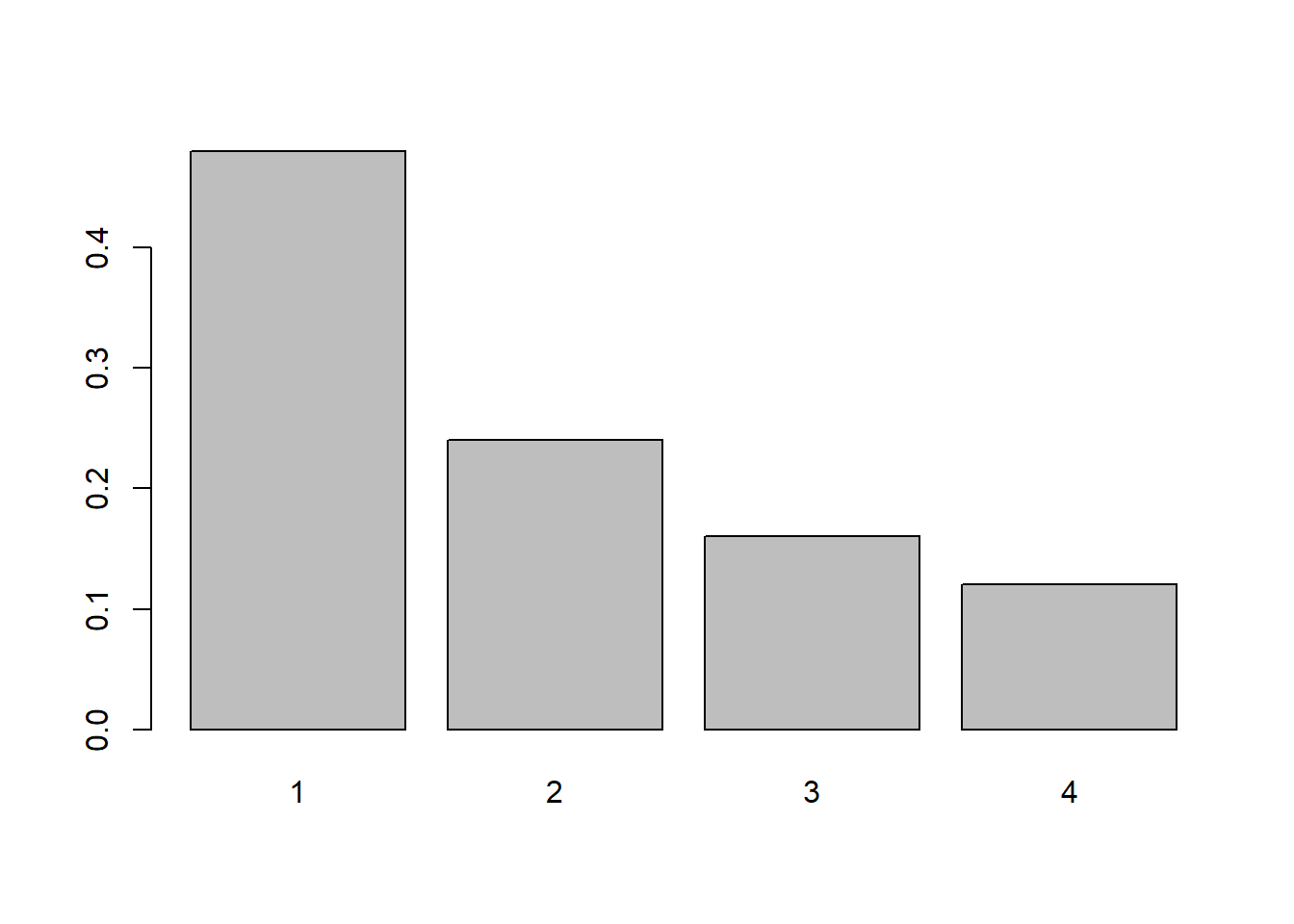

2. \(p_{k+1}=p_k/2\) for \(k=1,2,3\).

Solution

Starting with \(k=1\) we have \(p_2 = p_1/2\). Following this pattern, \(p_3=p_1/4\) and \(p_4=p_1/8\). If we add these together we have \(p_1(8/8 + 4/8 + 2/8 + 1/8) = 15/8\). Thus we have \(p_1=8/15, p_2=4/15, p_3=2/15\) and \(p_4=1/15\)

barplot(height=c(8/15, 4/15, 2/15, 1/15), names=1:4)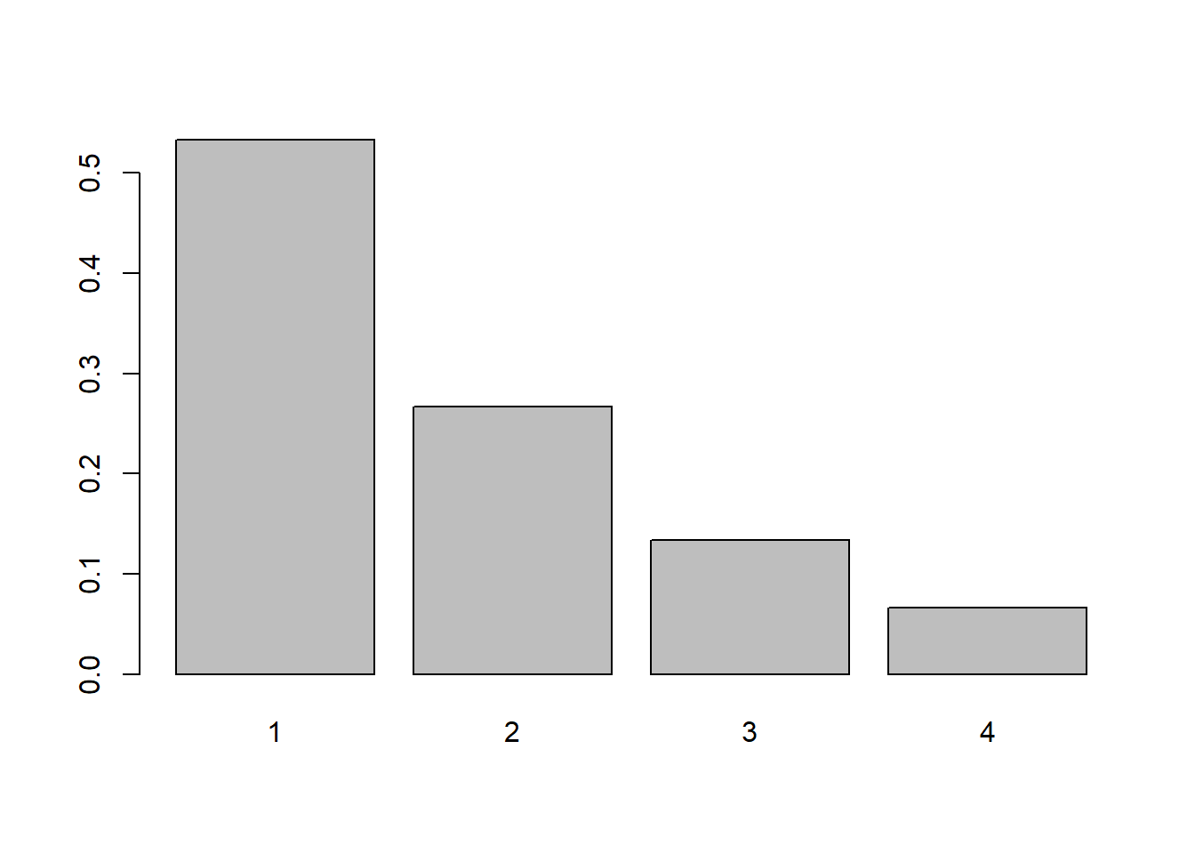

3. \(p_{k+1}=p_k/2^k\) for \(k=1,2,3\).

Solution

Starting with \(k=1\) we have \(p_2 = p_1/2\), \(p_3=p_2/2^2= p_2/4 = (p_1/2)/4 = p_1/8\). \(p_4 = p_3/2^3 = p_3/8 = (p_1/8)/8) = p_1/64\). The sum is \(p_1(64/64 + 32/64 + 8/64 + 1/64) = p_1(105/64)\) so \(p_1 = 64/105, p_2=32/105, p_3=8/105, p_4=1/105\)

barplot(height=c(64/105, 32/105, 8/105, 1/105), names=1:4)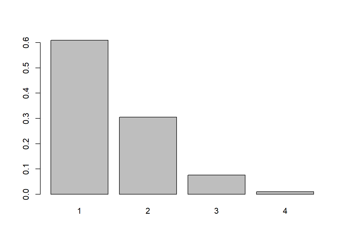

4. Can the random variables in parts a. through c. be extended to take on values in the set \(\{1,2,\ldots,\}\)? Why or why not? (Hint: You may use the fact that the series \(1+\frac12+\frac13+\cdots\) diverges.

Solution

Consider the pmf for part a. The sum of the probabilities would be \(\sum_{k=1}^\infty p_1/k\). However \(\sum_{k=1}^\infty \frac{1}{k}\) does not converge, so no matter what \(p_1\) is, the sum of probabilities will exceed 1.

For part b, the sum of the probabilities is \(\sum_{k=1}^\infty 2p_1/{2^{k}}\). Because \(\sum_{k=1}^\infty \frac{1}{2^k}=1\), then it would be possible to define a random variable with support \(1,2,\ldots\) with this pmf.

For part c, because \(p_k/2^k \leq p_k/2\), we at least know that \(\sum_k p_k\) is finite, so such a random variable with infinite support is certainly feasible. The exact value of \(p_1\) is not as simple to calculate, but we were not asked to do that.

6.22 Dice Difference

Two dice are tossed. Let \(X\) be the absolute difference in the number of dots facing up.

1. Find and plot the pmf of \(X\).

Solution

#It may be simplest to calculate all possible values of X. 
x <- vector("numeric")
for(i in 1:6){
  for(j in 1:6){
x[length(x)+1] = abs(i-j)
  }
}
#now that we have all equally likely values, we can just calculate the pmf in a prop.table
pX <- prop.table(table(x))
#And create a barplot.
barplot(pX)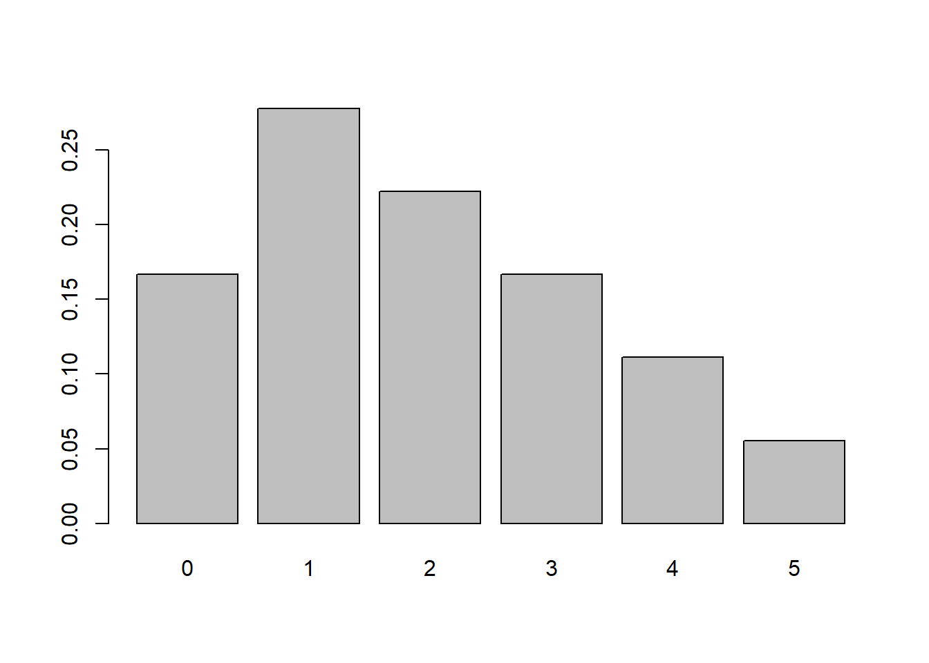

2. Find the probability that \(X\leq 2\).

Solution

#The probability that X <= 2 is easy to find using the pmf
#The columns are named with strings, so we can convert 0 1 and 2 to strings to pull out the proper probabilities.
sum(pX[as.character(0:2)])

[1] 0.6666667

3. Find \(\mathbb{E}X\) and \(\text{Var}X\).

Solution

#The expected value and variance can be calculated from the pmf.

(EX <- sum(0:5 * pX))

[1] 1.944444

(VarX <- sum((0:5 - EX)^2 * pX))

[1] 2.052469

#or by taking the mean and population variance of the x values themselves
mean(x)

[1] 1.944444

mean((x-mean(x))^2)

[1] 2.052469

6.23 Voltage random variable

A modem transmits a +2 voltage signal into a channel. The channel adds to this signal a noise term that is drawn from the set \(\{0,-1,-2,-3\}\) with respective probabilities \(\{4/10, 3/10, 2/10, 1/10\}\).

1. Find the pmf of the output \(Y\) of the channel.

Solution

#Let X be the noise
k <- seq(0,-3)
pk <- c(4/10, 3/10, 2/10, 1/10)

y <- sort(2+k)
py <- pk[order(2+k)]

barplot(height=py, names=y, main="pmf of Y")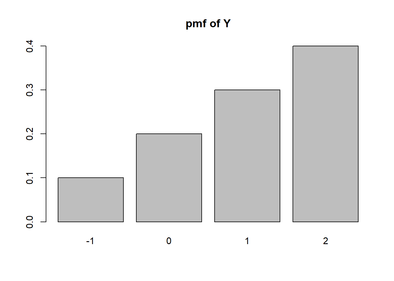

2. What is the probability that the channel’s output is equal to the input of the channel?

Solution

This happens when there’s no noise, with probability 4/10.

3. What is the probability that the channel’s output is positive?

Solution

#Interpreting 'positive' to be strictly positive, not zero:
sum(py[y>0])

[1] 0.7

4. Find the expected value and variance of \(Y\).

Solution

(EY <- sum(y*py))

[1] 1

(VarY <- sum((y-EY)^2*py))

[1] 1

6.24 Golf Score

On a given day, your golf score takes values from the numbers 1 through 10 with equal probability of getting each one. Assume that you play golf for three days, and assume that your three performances are independent. Let \(X_1, X_2\) and \(X_3\) be the scores that you get, and let \(X\) be the minimum of these three scores.

1. Show that for any discrete random variable \(X\) \(p_X(k)=\mathbb{P}(X > k-1) - \mathbb{P}(X>k)\).

Solution

\(P(X > k-1) = P(X \geq k) =P(X = k)+P(X > k)\), thus \(P(X=k)=P(X>k-1)-P(X>k)\).

2. What is the probability that \(\mathbb{P}(X_1>k)\) for \(k=1,\ldots,10\)?

Solution

\(P(X_1>k)=\frac{10-k}{10}\)

3. Use (a) to determine the pmf \(p_X(k)\) for \(k=1,\ldots,10\).

Solution

\(P(X > k) = P(X_1,X_2,X_3 > k) = P(X_1 > k)P(X_2>k)P(X_3>k)\)

This means \(P(X>k) =\frac{(10-k)^3}{10^3}\), and \(P(X>k-1)=\frac{(11-k)^3}{10^3}\). From the previous result, \(P(X=k)=P(X>k-1)-P(X>k)=\frac{(11-k)^3-(10-k)^3}{10^3}\)

4. What is the average score improvement if you play just for one day compared with playing for three days and taking the minimum?

Solution

This is asking to take the difference of the two expected values. It’s obvious that \(E(X_1)=5.5\); We need to find the expected value of \(X\).

x <- 1:10
px <- ((11-x)^3-(10-x)^3)/10^3
#double check
sum(px)

[1] 1

(EX <- sum(x*px))

[1] 3.025

5.5-EX

[1] 2.475

The average (expected) point improvement when going from a 1 day point to a minimum of 3 days is 2.475.

6.25 Functions of a random variable

Let \(g(X) = \begin{cases}1 & \text{if }X>10\\0 & \text{otherwise}\end{cases}\) and \(h(X) = \begin{cases}X-10 & \text{if }X-10>0\\0 & \text{otherwise}\end{cases}\)

1. For \(X \in S_X=\{1,2,\ldots,15\}\) with \(p_k = p_1/k\), find \(\mathbb{E}\left[g(X)\right]\)

Solution

k <- 1:15
p1 <- 1/(sum(1/k))
pk <- p1/k

g <- function(x){
  return(as.numeric(x>10))
}

sum(g(k)*pk)

[1] 0.1173098

2. For \(X \in S_X=\{1,2,\ldots,15\}\) with \(p_{k+1} = p_k/2\) (for \(k>1\)), find \(\mathbb{E}\left[h(X)\right]\).

Solution

h <- function(x){
  return(max(0, x-10))
}

p1 <- 1/(sum(1/2^(k-1)))
pk <- p1*(1/2^(k-1))

sum(h(k)*pk)

[1] 5

6.26 Voltage II

A voltage \(X\) is uniformly distributed on the set \(\{-3,\ldots,3,4\}\).

1. Find the mean and variance of \(X\).

Solution

x <- -3:4
px <- 1/length(x)

(EX <- sum(x*px))

[1] 0.5

(VarX <- sum((x-EX)^2*px))

[1] 5.25

2. Find the mean and variance of \(Y=-2X^2+3\).

Solution

y <- -2*x^2+3

(EY <- sum(y*px))

[1] -8

(VarY <- sum((y-EY)^2*px))

[1] 105

3. Find the mean and variance of \(W=\text{cos}(\pi X/8)\).

Solution

w <- cos(pi*x/8)
(EW <- sum(w*px))

[1] 0.6284174

(VarW <- sum((w-EW)^2*px))

[1] 0.1050915

4. Find the mean and variance of \(Z=\text{cos}^2(\pi X/8)\).

Solution

z <- w^2
(EZ <- sum(z*px))

[1] 0.5

(VarZ <- sum((z-EZ)^2*px))

[1] 0.125

6.27 A Continuous CDF

Consider a cdf

\(F_X(x)-\begin{cases}0,&\text{if }x < -1\\ 0.5 & \text{if }-1 \leq x < 0\\(1+x)/2 & \text{if }0 \leq x < 1\\1&\text{otherwise}\end{cases}\)

Find \(\mathbb{P}(X < -1)\), \(\mathbb{P}(-0.5 < X < 0.5)\), and \(\mathbb{P}(X>0.5)\).

Solution

#P(X < -1) = 0 because F(x) only goes up to .5 at x=-1, not when x < -1

#P(-.5 < X < .5) = F(.5) - F(-.5)
(1+.5)/2 - .5

[1] 0.25

#P(X > 0.5) = 1-P(X<.5) = 1-F(.5) 
1- (1+.5)/2

[1] 0.25

6.28 A Continuous CDF II

Let \(X\) have PDF \[f(x) = \begin{cases} 1-x/2,&0\leq x \leq 2\\0,&\text{otherwise}\end{cases}\]

1. Sketch the PDF and show geometrically that this is a valid PDF.

2. Find \(Pr[X>0]\) and \(Pr[X\geq 0]\)

3. Find \(Pr[X>1]\) and \(Pr[X\geq 1]\)

4. Use calculus or software to calculate the CDF from the PDF. Write the expression for \(F(x)\) and plot the PDF and CDF.

5. Use calculus or software to calculate the expected value of \(X\).

6.29 Two Random Variables

Suppose that \(X\) and \(Y\) are random variables with \(\mathbb{E}(X)=12\) and $(Y)=8.

1. Find \(\mathbb{E}(X-Y)\)
2. Find \(\mathbb{E}(5X-6Y)\)
3. Is it possible to determine \(\mathbb{E}(X^2)\) with the given information? Explain.

7 Beyond STAT 340

These problems are excellent practice but they are beyond the material we cover in STAT 340.

7.1 PMF Formula

Let \(X\) be a random variable with pmf \(p_k = c/2^k\) for \(k=1,2,\ldots\).

1. Determine the value of \(c\).

Solution

This was done above; because \(\sum_{i=1}^\infty 1/2^k = 1\), the value of \(c\) must be \(1\).

2. Find \(\mathbb{P}(X>4)\) and \(\mathbb{P}(6\leq X \leq 8)\).

Solution

\(P(X>4) = 1-P(X \leq 3)=1-(\frac12 + \frac14 + \frac18)\)

1-(1/2+1/4+1/8)

[1] 0.125

3. Find \(\mathbb{E}X\).

Solution

The expected value can be calculated by taking the sum \(\sum k p_k = \sum_{k=1}^\infty \frac{k}{2^k}\) which we can show using facts from calculus equals 2. Why? Well, as long as \(|p|<1, \sum_{k=1}^{\infty}p^k=\frac{p}{1-p}\) (this is a geometric series). If we take a derivative of both sides we get \(\sum_{k=1}^\infty kp^{k-1}=\frac{1}{(1-p)^2}\). Multiply both sides by \(p\) to get \(\sum_{k=1}^\infty kp^{k}=\frac{p}{(1-p)^2}\). In our case, \(p=\frac12\). Plugging this in we get \(\frac{.5}{.5^2}=2\).

7.2 PMF Formula II

Let \(X\) be a random variable with pmf \(p_k = c/2^k\) for \(k=-1,0,1,2,3,4,5\).

1. Determine the value of \(c\).

Solution

The sum of the probabilities are \(c(2 + 1 + \frac{1}{2}+\frac{1}{4}+\frac{1}8+\frac{1}{16}+\frac{1}{32})=c\frac{127}{32}\) so \(c=\frac{32}{127}\).

2. Find \(\mathbb{P}(1\leq X < 3)\) and \(\mathbb{P}(1 < X \leq 5)\).

Solution

c=32/127
k = seq(-1,5)
pk=c/2^k
names(pk) <- k
sum(pk[as.character(2)])

[1] 0.06299213

sum(pk[as.character(2:5)])

[1] 0.1181102

3. Find \(\mathbb{P}(X^3 < 5)\).

Solution

If \(X^3 < 5\) that means \(X^3 \leq 4\) and thus \(X \leq 4^{1/3}\approx 1.587\)

sum(pk[k<=4^(1/3)])

[1] 0.8818898

sum(pk[k^3<5])

[1] 0.8818898

4. Find the pmf and the cdf of \(X\).

Solution

barplot(height=pk, names=k, main='pmf of X')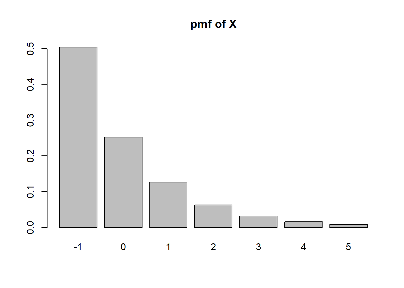

barplot(height=cumsum(pk), names=k, main='cdf of X')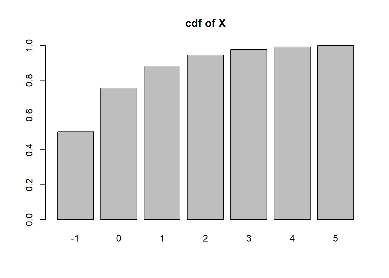

7.3 Properties of Expectation I

For a continuous random variable \(X\) and constant \(c\), prove that \(\mathbb{E}(cX)=c\mathbb{E}(X)\)

7.4 Properties of Expectation II

For a continuous random variable \(X\) and constants \(a,b\), prove that \(\mathbb{E}(aX+b)=a\mathbb{E}(X)+b\)

7.5 Variance of a RV from the pmf

Let \(X\) be a random variable with pmf \(p_k = 1/2^k\) for \(k=1,2,\ldots\).

1. Find \(\text{Var}X\).

Solution

The variance is \(E(X^2)-(EX)^2=E(X^2)-4\). The expected value of \(X^2\) can be derived, though it’s not so fun…

Start by taking the equation \(\sum_k kp^k = \frac{p}{(1-p)^2}\) and take a derivative again. We get \(\sum_k k^2 p^{k-1} = \frac{(1-p)^2+2p(1-p)}{(1-p)^4}\). Multiply through by \(p\) to get \(\sum_k k^2 p^k = \frac{p(1-p)^2+2p^2(1-p)}{(1-p)^4}\). If we let \(p=\frac12\) we have found \(E(X^2)=\sum_{k=1}^\infty k^2(\frac12)^k=\dfrac{\frac18-\frac{2}{8}}{\frac{1}{16}}=6\). Thus \(Var(X)=E(X^2)-E(X)^2 = 6-4=2\). It should be noted that this random variable is actually a geometric random variable (well, according to the “number of trials until and including the first success definition). If we define \(Y\sim Geom(.5)\) using our definition of “number of failures before the first success” then We can let \(X=Y+1\). \(E(X)=E(Y+1)=\frac{1-.5}{.5}+1=2\) and \(Var(X)=Var(Y)=\frac{1-p}{p2}=\frac{.5}{.25^2}=2\).

7.6 Variance Formula

Show that \(\mathbb{E}(X-\mu)^2 = \mathbb{E}X^2-\mu^2\). Hint: expand the quantity \((X-\mu)^2\) and distribute the expectation over the resulting terms.

Solution

The proof goes like this: We first FOIL \((X-\mu)^2\):

\(\mathbb{E}(X-\mu)^2 = \mathbb{E}(X^2 - 2\mu X + \mu^2)\)

We next split the expected value into 3 expected values using the fact that \(\mathbb{E}\) is a linear operator.

\(\mathbb{E}(X-\mu)^2 = \mathbb{E}X^2 -2\mu \mathbb{E}X + \mathbb{E}\mu^2\)

We next observe that \(\mu^2\) is constant and \(\mathbb{X}=\mu\)

\(\mathbb{E}(X-\mu)^2 = \mathbb{E}X^2 -2\mu \mu + \mu^2\)

We can simplify the expression and we’re done!