3 Probability and Random Variables
These notes will discuss the most fundamental object in statistics: random variables.
We use random variables, within the framework of probability theory, to model how our data came to be.
We will first introduce the idea of a random variable (and its associated distribution) and review probability theory.
We also explore the concept of independence of random variables. We will discuss in more detail what it means for variables to be independent, and we will discuss the related notion of correlation.
We will also see how independence relates to “conditional probability”, and how we can use this different “kind” of probability to answer questions that frequently arise in statistics (especially in medical trials) by appealing to Bayes’ rule.
3.1 Learning objectives
After this lesson, you will be able to
- Compute the probabilities of simple events under different probability distributions using R.
- Explain what a random variable is
- Explain what it means for variables to be dependent or independent and assess how reasonable independence assumptions are in simple statistical models.
- Explain expectations and variances of sums of variables are influenced by the dependence or independence of those random variables.
- Explain correlation, compute the correlation of two random variables, and explain the difference between correlation and dependence.
- Define the conditional probability of an event \(A\) given an event \(B\) and calculate this probability given the appropriate joint distribution.
- Use Bayes’ rule to compute \(\Pr[B \mid A]\) in terms of \(\Pr[A \mid B]\), \(\Pr[A]\) and \(\Pr[B]\).
3.2 Probability refresher
A random experiment (or random process) is a procedure which produces an uncertain outcome. The set of possible outcomes is often denoted \(\Omega\).
- When we flip a coin, it can land either heads (\(H\)) or tails (\(T\)), so the outcomes are \(\Omega = \{H, T\}\).
- When we roll a six-sided die, there are six possible outcomes, \(\Omega = \{1,2,3,4,5,6\}\).
- In other settings, the outcomes might be an infinite set.
- Ex: if we measure the depth of Lake Mendota, the outcome may be any positive real number (theoretically)
Usually \(\Omega\) will is discrete (e.g., \(\{1,2,\dots\}\)) or continuous (e.g., \([0,1]\)). We call the associated random variable discrete or continuous, respectively.
A subset \(E \subseteq \Omega\) of the outcome space is called an event.
A probability is a function that maps events to numbers, with the properties that
- \(\Pr[ E ] \in [0,1]\) for all events \(E\)
- \(\Pr[ \Omega ] = 1\)
- For \(E_1,E_2 \subseteq \Omega\) with \(E_1 \cap E_2 = \emptyset\), \(\Pr[ E_1 \cup E_2 ] = \Pr[ E_1 ] + \Pr[ E_2 ]\)
If \(\Pr[E_1 \cap E_2]=0\), we say that \(E_1\) and \(E_2\) are mutually exclusive (or disjoint)
Two events \(E_1\) and \(E_2\) are independent if \(\Pr[ E_1 \cap E_2 ] = \Pr[ E_1 ] \Pr[ E_2 ]\).
3.2.1 Example: Coin flipping
Consider a coin toss, in which the possible outcomes are \(\Omega = \{ H, T \}\).
This is a discrete random experiment. If we have a fair coin, then it is sensible that \(\Pr[ X=1 ] = \Pr[ X=0 ] = 1/2\).
Exercise (optional): verify that this probability satisfies the above properties!
We will see in a later lecture that this is a special case of a Bernoulli random variable, which you are probably already familiar with.
3.2.2 Example: Six-sided die
If we roll a die, the outcome space is \(\Omega = \{1,2,3,4,5,6\}\), and the events are all the subsets of this six-element set.
So, for example, we can talk about the event that we roll an odd number \(E_{\text{odd}} = \{1,3,5\}\) or the event that we roll a number larger than \(4\), \(E_{>4} = \{5,6\}\).
3.2.3 Example: Human heights
We pick a random person and measure their height in, say, centimeters. What is the outcome space?
- One option: the outcome space is the set of positive reals, in which case this is a continuous random variable.
- Alternatively, we could assume that the outcome space is the set of all real numbers.
Highlight: the importance of specifying our assumptions and the outcome space we are working with in a particular problem.
3.2.4 A note on models, assumptions and approximations
Note that we are already making an approximation– our outcome sets aren’t really exhaustive, here.
- When you toss a coin, there are possible outcomes other than heads and tails: it is technically possible to land on the edge.
- Similarly, perhaps the die lands on its edge.
Human heights:
- We can only measure a height to some finite precision (say, two decimal places), so it is a bit silly to take the outcome space to be the real numbers.
- After all, if we can only measure a height to two decimal places, then there is no way to ever obtain the event, “height is 160.3333333… centimeters”.
Good to be aware of these approximations - but they usually won’t bother us.
3.3 Events and independence.
Two events \(E_1\) and \(E_2\) are independent if \(\Pr[ E_1 \cap E_2 ] = \Pr[ E_1 ] \Pr[ E_2 ]\).
We may write \(\Pr[ E_1, E_2]\) to mean \(\Pr[ E_1 \cap E_2 ]\), read as “the probability of events \(E_1\) and \(E_2\)” or “the probability that \(E_1\) and \(E_2\) occur”.
- For example, if each of us flip a coin, it is reasonable to model them as being independent.
- Learning whether my coin landed heads or tails doesn’t tell us anything about your coin.
3.3.1 Example: dice and coins
Suppose that you roll a die and I flip a coin. Let \(D\) denote the (random) outcome of the die roll, and let \(C\) denote the (random) outcome of the coin flip. So \(D \in \{1,2,3,4,5,6\}\) and \(C \in \{1,0\}\). Suppose that for all \(d \in \{1,2,3,4,5,6\}\) and all \(c \in \{1,0\}\), \(\Pr[ D=d, C=c ] = 1/12\).
Question: Verify that the random variables \(D\) and \(C\) are independent, or at least check that it’s true for two particular events \(E_1 \subseteq \{1,2,3,4,5,6\}\) and \(E_2 \subseteq \{1,0\}\).
3.3.2 Example: more dice
Suppose that we roll a fair six-sided die. Consider the following two events: \[ \begin{aligned} E_1 &= \{ \text{The die lands on an even number} \} \\ E_2 &= \{ \text{The die lands showing 3} \}. \end{aligned} \]
Are these two events independent? If I tell you that the die landed on an even number, then it’s certainly impossible that it landed showing a 3, since 3 isn’t even. These events should not be independent.
Let’s verify that \[ \Pr[ E_1 \cap E_2 ] \neq \Pr[ E_1 ] \Pr[ E_2 ]. \]
There are six sides on our die, numbered 1, 2, 3, 4, 5, 6, and three of those sides are even numbers, so \(\Pr[ E_1 ] = 1/2\).
The probability that the die lands showing 3 is exactly \(\Pr[ E_2 ] = 1/6\).
Putting these together, \(\Pr[E_1] \Pr[E_2] = 1/12\).
On the other hand, let’s consider \(E_1 \cap E_2\) (the die is even and it lands showing three). These two events cannot both happen!
That means that \(E_1 \cap E_2 = \emptyset\). Thus \(\Pr[ \emptyset ] = 0.\)
(Aside: why? Hint: \(\Pr[ \Omega ] = 1\) and \(\emptyset \cap \Omega = \emptyset\); now use the fact that the probability of the union of disjoint events is the sum of their probabilities).
So we have \[ \Pr[ E_1 \cap E_2 ] = 0 \neq \frac{1}{12} =\Pr[ E_1 ] \Pr[ E_2 ]. \]
Our two events are indeed not independent.
3.3.3 Mutually Exclusive vs Independent
Two events \(E_1\) and \(E_2\) are mutually exclusive if the probability of both occurring simultaneously is zero \[P(E_1 \cap E_2) = 0\]
Could two events \(E_1\) and \(E_2\) with non-zero probabilities be mutually exclusive and independent? Think about it!
3.4 Conditional probability
We can’t talk about events and independence without discussing conditional probability.
To motivate this, consider the following: suppose I roll a six-sided die. What is the probability that the die lands showing 2?
Now, suppose that I don’t tell you the number on the die, but I do tell you that the die landed on an even number (i.e., one of 2, 4 or 6). Now what is the probability that the die is showing 2?
We can work out the probabilities by simply counting possible outcomes. Are the probabilities the same?
3.4.1 Example: disease screening
Here’s a more real-world (and more consequential example): suppose we are screening for a rare disease. A patient takes the screening test, and tests positive. What is the probability that the patient has the disease, given that they have tested positive for it?
We will need to establish the rules of conditional probability before we can tackle a problem such as this.
3.4.2 Introducing conditional probability
These kinds of questions, in which we want to ask about the probability of an event given that something else has happened, require that we be able to define a “new kind” of probability, called conditional probability.
Let \(A\) and \(B\) be two events.
- Example: \(A\) could be the event that a die lands showing 2 and \(B\) is the event that the die landed on an even number.
- Example: \(A\) could be the event that our patient has a disease and \(B\) is the event that the patient tests positive on a screening test.
Provided that \(\Pr[ B ] > 0\), we define the conditional probability of \(A\) given \(B\), written \(\Pr[ A \mid B]\), according to \[ \Pr[ A \mid B ] = \frac{ \Pr[ A \cap B ] }{ \Pr[ B ] }. \] Note that if \(\Pr[B] = 0\), then the ratio on the right-hand side is not defined, hence why we demanded that \(\Pr[B] > 0\).
Let’s try computing one of these conditional probabilities: what is the probability that the die is showing 2 conditional on the fact that it landed on an even number?
Well,
- \(\Pr[ \text{ even } ] = 1/2\), because there are three even numbers on the die, and all six numbers are equally likely: \(3/6 = 1/2\).
- \(\Pr[ \text{ die lands 2 } \cap \text{even} ] = \Pr[ \text{ die lands 2 }]\), since \(2\) is an even number.
So the conditional probability is \[ \begin{aligned} \Pr[ \text{ die lands 2 } \mid \text{ even }] &= \frac{ \Pr[ \text{ die lands 2 } \cap \text{even} ] }{ \Pr[ \text{ even } ] } \\ &= \frac{ \Pr[ \text{ die lands 2 }]} { \Pr[ \text{ even } ] } \\ &= \frac{ 1/6 }{ 1/2 } = 1/3. \end{aligned} \] This makes sense– given that the die lands on an even number, we are choosing from among three outcomes: \(\{2,4,6\}\). The probability that we choose \(2\) from among these three possible equally-likely outcomes is \(1/3\).
3.4.3 Example: disease screening (continued)
What about our disease testing example? What is the probability that our patient has the disease given that they tested positive?
Well, applying the definition of conditional probability, \[ \Pr[ \text{ disease} \mid \text{ positive test }] = \frac{ \Pr[ \text{ disease} \cap \text{ positive test }] }{ \Pr[ \text{positive test} ] } \]
Okay, but what is \(\Pr[ \text{ positive test} ]\)? I guess it’s just the probability that a random person (with the disease or not) tests positive? For that matter, what is \(\Pr[ \text{ disease} \cap \text{ positive test }]\)? These can be hard events to assign probabilities to! Luckily, there is a famous equation that often gives us a way forward.
3.4.4 Bayes’ rule
The Reverend Thomas Bayes was the first to suggest an answer to this issue. Bayes’ rule, as it is now called, tells us how to relate \(\Pr[ A \mid B]\) to \(\Pr[ B \mid A]\): \[ \Pr[ A \mid B ] = \frac{ \Pr[ B \mid A ] \Pr[ A ]}{ \Pr[ B ]}. \]
This is useful, because it is often easier to write one or the other of these two probabilities.
Applying this to our disease screening example, \[ \Pr[ \text{ disease} \mid \text{ positive test }] = \frac{ \Pr[\text{ positive test } \mid \text{ disease}] \Pr[ \text{ disease}]} { \Pr[ \text{ positive test } ] } \]
The advantage of using Bayes’ rule in this context is that the probabilities appearing on the right-hand side are all straight-forward to think about (and estimate!).
- \(\Pr[ \text{ disease}]\) is the just the probability that a randomly-selected person has the disease. This is known as the prevelance of the diseases in the population. We could estimate this probability by randomly selecting a random group of people and determining if they have the disease (hopefully not using the screening test we are already using…).
- \(\Pr[\text{ positive test } \mid \text{ disease}]\) is the probability that when we give our screening test to a patient who has the disease in question, the test returns positive. This is often called the sensitivity of a test, a term you may recall hearing frequently in the early days of the COVID-19 pandemic.
- \(\Pr[ \text{ positive test } ]\) is just the probability that a test given to a (presumably randomly selected) person returns a positive result. We just said about that this is the hard thing to estimate.
3.4.5 Example: testing for a rare disease
Suppose that we are testing for a rare disease, say, \[ \Pr[ \text{ disease}] = \frac{1}{10^6}, \]
and suppose that a positive test is also rare, in keeping with the fact that our disease is rare and our test presumably has a low false positive rate: \[ \Pr[ \text{ positive test} ] = 1.999*10^{-6} \] Note that this probability actually depends on the sensitivity \(\Pr[\text{ positive test } \mid \text{ disease}]\) and the specificity \(1-\Pr[\text{ positive test } \mid \text{ healthy}]\) of our test. You’ll explore this part more on your homework, but we’re just going to take this number as given for now.
Finally, let’s suppose that our test is 99.99% accurate: \[ \Pr[\text{ positive test } \mid \text{ disease}] = 0.9999 = 1-10^{-4} \]
To recap, \[ \begin{aligned} \Pr[ \text{ disease}] &= \frac{1}{10^6} \\ \Pr[ \text{ positive test} ] &= 1.999*10^{-6} \\ \Pr[\text{ positive test } \mid \text{ disease}] &= 0.9999. \end{aligned} \]
Now, suppose that a patient is given the screening test and receives a positive result. Bayes’ rule tells us \[ \begin{aligned} \Pr[ \text{ disease} \mid \text{ positive test }] &= \frac{ \Pr[\text{ positive test } \mid \text{ disease}] \Pr[ \text{ disease}]} { \Pr[ \text{ positive test } ] } = \frac{ 0.9999 * 10^{-6} }{ 1.999*10^{-6} } \\ &= 0.5002001. \end{aligned} \]
So even in light of our positive screening test result, the probability that our patient has the disease in question is still only about 50%!
This is part of why, especially early on in the pandemic when COVID-19 was especially rare, testing for the disease in the absence of symptoms was not considered especially useful.
More generally, this is why most screenings for rare diseases are not done routinely– doctors typically screen for rare diseases only if they have a reason to think a patient is more likely to have that disease for other reasons (e.g., family history of a genetic condition or recent exposure to an infectious disease).
3.4.6 Calculating the denominator in Bayes’ Rule
The denominator can be decomposed into two parts using a property known as the Law of Total Probability.
\[ \Pr[ \text{ positive test} ] = \Pr[ \text{ positive test} \cap \text{disease}]+\Pr[ \text{ positive test} \cap \text{no disease}] \]
In other words, all positive results are either true positives or false positives. Because these are mutually exclusive events, the total probability of a positive result is the probability of a true positive plus the probability of a false positive. We can expand each of these terms using the conditional probability rule.
\[ \Pr[ \text{ positive test} \cap \text{disease}] = \Pr[\text{ positive test } \mid \text{ disease}] \Pr[ \text{ disease}] \] \[ \Pr[ \text{ positive test} \cap \text{no disease}] = \Pr[\text{ positive test } \mid \text{ no disease}] \Pr[ \text{no disease}] \]
For example, suppose that a genetic condition occurs in roughly 1 out of 800 individuals. A simple saliva test is available. If a person has the gene, the test is positive with 97% probability. If a person does not have the gene, a false positive occurs with 4% probability.
To simplify notation, let \(G\) represent “the individual has the gene” and \(G'\) be the complementary event that “the individual does not have the gene.” Furthermore, let \(Pos\) and \(Neg\) represent the test results.
If a random person from the population takes the test and gets a positive result, what is the probability they have the genetic condition?
Bayes’ Rule to the rescue:
\[ \begin{aligned} P[G | Pos] &= \dfrac{P[Pos | G] P[G]}{P[Pos | G] P[G] + P[Pos | G'] P[G']}\\ &= \dfrac{(.97)(1/800)}{(.97)(1/800)+(.04)(799/800)}\\ &\approx 0.0295 \end{aligned} \] In other words, a positive test result would raise the likelihood of the gene being present from \(1/800=0.00125\) up to \(.0295\).
3.4.7 Dependent free throw shots
Suppose a basketball player’s likelihood of making a basket when making a free throw depends on the previous attempt. On the first throw, they have a probability of \(0.67\) of making the basket. On the second throw, following a basket the probability goes up to \(.75\). If the first throw is a miss, the probability of a basket on the second throw goes down to \(0.62\).
Exercise: If the second throw is a basket, what is the likelihood the first throw is a basket?
Exercise: Given that the player scores at least 1 point, what is the probability that they score 2 points total?
3.5 Random Variables
Consider the following quantities/events:
- Whether or not a coin flip comes up heads or tails.
- How many people in the treatment group of a vaccine trial are hospitalized.
- The water level measured in Lake Mendota on a given day.
- How many customers arrive at a store between 2pm and 3pm today.
- How many days between installing a lightbulb and when it burns out.
All of these are examples of events that we might reasonably model according to different random variables.
Informal definition of a random variable: a (random) number \(X\) about which we can compute quantities of the form \(\Pr[ X \in S ]\), where \(S\) is a set.
3.5.1 Random variables (formal definition)
A random variable \(X\) is specified by an outcome set \(\Omega\) and a function that specifies probabilities of the form \(\Pr[ X \in E ]\) where \(E \subseteq \Omega\) is an event. For our purposes though it’s helpful to think of a random variable as a variable that can take random values with specified probabilities.
Broadly speaking random variables fall into two categories: discrete and continuous. A discrete random variable can take a value from a countable set (for example, the integers). The set of possible values could be finite or possibly infinite. A continuous random variable can take any real number value along an interval (or union of intervals).
3.5.2 Discrete Random Variables
3.5.2.1 Probability Mass Function
To define a discrete random variable it is enough to define a function mapping possible values to their probabilities. This is known as a probability mass function (pmf). It can be represented in a table or mathematically.
For example, suppose the random variable \(X\) can take values \(0,1,2,3\) or \(4\). We could define the probability mass function using a table:
| \(k\) | 0 | 1 | 2 | 3 | 4 |
| \(Pr[X=k]\) | .10 | .15 | .20 | .30 | .25 |
Another random variable \(Y\) may be defined as taking any non-negative integer \(k\geq0\), with \[Pr[Y=k]=(.6)(.4^k)\]
3.5.2.2 The Cumulative Distribution Function
We are often interested not just in the probability that a random variable \(X\) takes one particular value \(k\), but a value within a range. From a probability mass function \(f(k)=Pr[X=k]\) we can define a cumulative distribution function (cdf) \(F(k)\). \[F(k) = Pr[X \leq k] = \sum_{x \leq k}Pr[X=x]\] (we can just add up these probabilities since they are disjoint events).
3.5.2.3 CDF example
For example, we can expand the pmf from the previous example to a cdf.
| \(k\) | 0 | 1 | 2 | 3 | 4 |
| \(Pr[X=k]\) | .10 | .15 | .20 | .30 | .25 |
| \(F(k)\) | .10 | .25 | .45 | .76 | 1.0 |
Notice that the cdf increases (technically it is “non-decreasing”) as \(k\) increases, going from 0 to 1 and no higher. While the table above only gives cdf values for integers, it is technically a step function defined for all real numbers. The cdf would be 0 for any value \(k\) lower than the lowest possible value of \(X\).
3.6 Expectation
Before we continue with more random variables, let’s take a pause to discuss one more important probability concept: expectation. You will hopefully recall from previous courses in probability and/or statistics the notion of expectation of a random variable.
Expectation: long-run averages
The expectation of a random variable \(X\), which we write \(\mathbb{E} X\), is the “long-run average” of the random variable.
What we would see on average if we observed many realizations of \(X\).
That is, we observe \(X_1,X_2,\dots,X_n\), and consider their average, \(\bar{X} = n^{-1} \sum_{i=1}^n X_i\).
3.6.1 Expected value and the Law of Large Numbers (first peek)
The law of large numbers (LLN) states that in a certain sense, as \(n\) gets large, \(\bar{X}\) gets very close to \(\mathbb{E} X\).
We would like to say something like \[ \lim_{n \rightarrow \infty} \frac{1}{n} \sum_{i=1}^n X_i = \mathbb{E} X. \] But \(n^{-1} \sum_i X_i\) is a random sum, so how can we take a limit?
Roughly speaking, for \(n\) large, with high probability, \(\bar{X}\) is close to \(\mathbb{E}\).
3.6.2 Expectation: formal definition
More formally, if \(X\) is a discrete random variable, we define its expectation to be \[ \mathbb{E} X = \sum_k k \Pr[ X = k], \] where the sum is over all \(k\) such that \(\Pr[ X=k ] > 0\).
- Note that this set could be finite or infinite.
- If the set is infinite, the sum might not converge, in which case we say that the expectation is either infinite or doesn’t exist. But that won’t be an issue this semester.
Question: can you see how this definition is indeed like the “average behavior” of \(X\)?
3.6.3 Example: Calculating Expectation
Calculate the expected value of the random variable \(X\) with the pmf
| \(k\) | 0 | 1 | 2 | 3 | 4 |
| \(Pr[X=k]\) | .10 | .15 | .20 | .30 | .25 |
3.6.4 LLN Important take-away
The law of large numbers says that if we take the average of a bunch of independent RVs, the average will be close to the expected value.
- Sometimes it’s hard to compute the expected value exactly (e.g., because the math is hard– not all sums are nice!)
- This is where Monte Carlo methods come in– instead of trying to compute the expectation exactly, we just generate lots of RVs and take their average!
- If we generate enough RVs, the LLN says we can get as close as we want.
- We’ll have lots to say about this in our lectures on Monte Carlo methods next week.
3.7 Continuous random variables
Continuous random variables, which take values in “continuous” sets like the interval \([0,1]\) or the real \(\mathbb{R}\).
Continuous random variables have probability density functions, which we will usually write as \(f(x)\) or \(f(t)\).
These random variables are a little trickier to think about at first, because it doesn’t make sense to ask about the probability that a continuous random variable takes a specific value. That is, \(\Pr[ X = k ]\) doesn’t really make sense when \(X\) is continuous (actually– in a precise sense this does make sense, but the probability is always zero; you’ll see why below).
3.7.1 The probability density function
Rather than defining the probability measure for specific values \(k\) that the random variable can take, it only makes sense to describe the relative likelihood of different values. We use a probability density function (pdf) to do this. The pdf, typically denoted \(f(x)\) defines the how much probability per unit is to be found at \(X=x\).
Let’s look at an example.
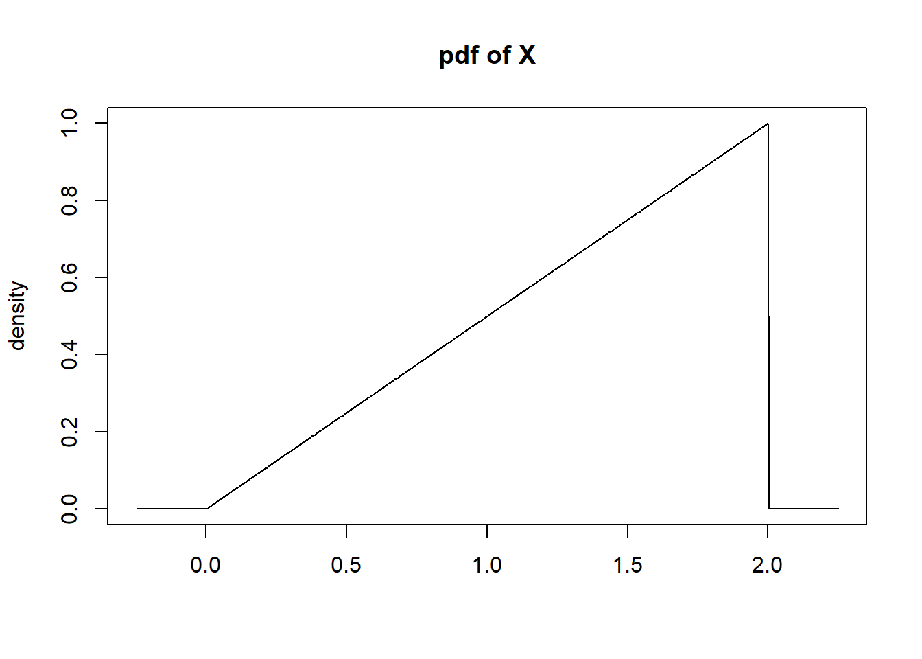
3.7.2 PDF Example
Define continuous rv \(X\) with density function \(f(x)=.5x\) for \(x \in [0,2]\).
3.7.3 Calculating probabilities for continuous RVs
Probability can be calculated by integration: For some interval \([a,b]\) we calculate \[Pr\left[a\leq X\leq b\right] = \int_a^b f(x)dx\]
Because the definite integral correspond to the area under the curve, we can sometimes find probabilities using geometry rather than calculus.
Example: Calculate \(Pr[.5 \leq X \leq 1.5]\).
3.7.4 Probability that X=k?
Because of how we define probability for continuous random variables, \(Pr[X=k]=\int_k^k f(x)dx=0\), so there is no measurable probability for any one particular value for a continuous random variable. Therefore we can say \(Pr[X < k]\) or \(Pr[X \leq k]\). It doesn’t matter since \(Pr[X=k]=0\).
3.7.5 CDF for a continuous random variable
The CDF is defined as \(F(x) = Pr[X \leq x]\) (using \(x\) instead of \(k\) for now). This is the same definition for continuous random variables, but mathematically it arises from an integral rather than a summation: \[F(x) = Pr[X \leq x] = \int_{-\infty}^x f(t)dt\] For this course we won’t be integrating density functions. On occasion you’ll be provided with a cdf but you won’t have to produce them yourself.
But it’s worth noting that \(F(x) \in [0,1]\) for all random variables, and \(F(x)\) is a non-decreasing function, with \(F(x)\to0\) as \(x \to -\infty\), and \(F(x)\to 1\) as \(x \to +\infty\).
3.7.6 Expectation for continuous random variables
Previously, we defined the expectation of a discrete random variable \(X\) to be \[ \mathbb{E} X = \sum_k k \Pr[ X = k ], \] with the summand \(k\) ranging over all allowable values of \(X\). When \(X\) is continuous how should we define the expectation? Change the sum to an integral!
\[ \mathbb{E} X = \int_\Omega t f(t) dt, \]
where \(f(t)\) is the density of \(X\) and \(\Omega\) is the support.
This type of exercise is best left to another statistics course. For us it’s enough to think of the expectation as a balancing point (center of mass) for a continuous random variable’s distribution function.
3.8 Random Variables and Independence
Two random variables \(X\) and \(Y\) are independent if for all sets \(S_1,S_2\), we have \(\Pr[ X \in S_1 ~\&~ Y \in S_2 ] = \Pr[ X \in S_1 ] \Pr[ Y \in S_2 ]\).
Roughly speaking, two random variables are independent if learning information about one of them doesn’t tell you anything about the other.
- For example, if each of us flips a coin, it is reasonable to model them as being independent.
- Learning whether my coin landed heads or tails doesn’t tell us anything about your coin.
3.8.1 Independent Random Variables
Informally, we’ll say that two random variables \(X\) and \(Y\) are independent if any two events concerning those random variables are independent.
That is, for any event \(E_X\) concerning \(X\) (i.e., \(E_X = \{ X \in S \}\) for \(S \subseteq \Omega)\) and any event \(E_Y\) concerning \(Y\), the events \(E_X\) and \(E_Y\) are independent.
i.e., if two random variables \(X\) and \(Y\) are independent, then for any two sets \(S_1, S_2 \subset \Omega\), \[ \Pr[ X \in S_1, Y \in S_2 ] = \Pr[ X \in S_1] \Pr[ Y \in S_2 ]. \]
If \(X\) and \(Y\) are both discrete, then for any \(k\) and \(\ell\), \[ \Pr[ X=k, Y=\ell ] = \Pr[ X=k ] \Pr[ Y=\ell ]. \]
Similarly, if \(X\) and \(Y\) are continuous, then the joint density has the same property: \[ f_{X,Y}(s,t) = f_X(s) f_Y(t). \]
3.8.2 How reasonable is independence?
In most applications, it is pretty standard that we assume that our data are drawn independently and identically distributed according to some distribution. We say “i.i.d.”. For example, if \(X_1, X_2, \ldots, X_n\) are all continuous uniform random variables between 0 and 1, we would say \[ X_i \overset{\text{iid}}{\sim} \text{Uniform}(0,1), \text{ for } i=1,\ldots, n \]
This notation is common to denote iid random variables.
As another example, when we perform regression (as you did in STAT240, and which we’ll revisit in more detail later this semester), we imagine that the observations (i.e., predictor-response pairs) \((X_1,Y_1),(X_2,Y_2),\dots,(X_n,Y_n)\) are independent.
Most standard testing procedures (e.g., the t-test) assume that data are drawn i.i.d.
How reasonable are these assumptions?
It depends on where the data comes from! We have to draw on what we know about the data, either from our own knowledge or from that of our clients, to assess what assumptions are and aren’t reasonable.
Like most modeling assumptions, we usually acknowledge that independence may not be exactly true, but it’s often a good approximation to the truth!
Example: suppose we are modeling the value of a stock over time. We model the stock’s price on days 1, 2, 3, etc as \(X_1, X_2, X_3, \dots\). What is wrong with modeling these prices as being independent of one another? Why might it still be a reasonable modeling assumption?
What if instead we look at the change in stock price from day to day? For example, let \(Y_i = X_{i+1}-X_{i}\). In other words, \(X_{i+1}=X_i+Y_i\). Would it be more reasonable to assume that the \(Y_i\)’s are independent?
What if instead of considering a stock’s returns on one day after another, we look at a change in stock price on one day, then at the change 10 days from that, and 10 days from that, and so on? Surely there is still dependence, but a longer time lag between observations might make us more willing to accept that our observations are close to independent (or at least have much smaller covariance!).
Note: Tobler’s first law of geography states ‘Everything is related to everything else, but near things are more related than distant things.’ Does that ring true in this context?
Example: suppose we randomly sample 1000 UW-Madison students to participate in a survey, and record their responses as \(X_1,X_2,\dots,X_{1000}\). What might be the problem with modeling these responses as being independent? Why might be still be a reasonable modeling assumption?
3.8.3 (in)dependence, expectation and variance
Recall the definition of the expectation: If \(X\) is continuous with density \(f_X\), \[ \mathbb{E} X = \int_\Omega t f_X(t) dt, \]
and if \(X\) is discrete with probability mass function \(\Pr[ X=k]\), \[ \mathbb{E} X = \sum_{k \in \Omega} k \Pr[X=k] \]
With the expectation defined, we can also define the variance, \[ \operatorname{Var} X = \mathbb{E} (X - \mathbb{E} X)^2 = \mathbb{E} X^2 - \mathbb{E}^2 X. \]
That second equality isn’t necessarily obvious– we’ll see why it’s true in a moment.
Note: we often write \(\mathbb{E}^2 X\) as short for \((\mathbb{E} X)^2\).
A basic property of expectation is that it is linear. For any constants (i.e., non-random) \(a,b \in \mathbb{R}\), \[ \mathbb{E} (a X + b) = a \mathbb{E} X + b. \] If \(X,Y\) are random variables, then \[ \mathbb{E}( X + Y) = \mathbb{E} X + \mathbb{E} Y. \]
Note that derivatives and integrals are linear, too. For example, \[ (a ~f(t) + b ~g(t))' = a ~ f'(t) + b ~g'(t) \]
and \[ \int(a f(t) + b g(t)) dt = a \int f(t) dt + b \int g(t) dt \]
Because expected value is simply an integral (or summation), the linearity of expectation follows directly from the definition.
Exercise: prove that \(\mathbb{E} (a X + b) = a \mathbb{E} X + b\) for discrete r.v. \(X\).
Exercise: prove that \(\mathbb{E}( X + Y) = \mathbb{E} X + \mathbb{E} Y\) for discrete \(X\) and \(Y\).
Exercise: Use the linearity of expectation to prove that \(\mathbb{E} (X - \mathbb{E} X)^2 = \mathbb{E} X^2 - \mathbb{E}^2 X\). Hint: \(\mathbb{E}( X \mathbb{E} X) = \mathbb{E}^2 X\) because \(\mathbb{E} X\) is NOT random– it pops right out of the expectation just like \(a\) does in the equation above.
The definition of variance and the linearity of expectation are enough to give us a property of variance:
For any constants (i.e., non-random) \(a,b \in \mathbb{R}\), \[ \operatorname{Var} (a X + b) = a^2 \operatorname{Var} (X). \]
Exercise: Use the definition \(\operatorname{Var}(X)=\mathbb{E} X^2 - \mathbb{E}^2 X\) to prove the above.
This linearity property implies that the expectation of a sum is the sum of the expectations: \[ \mathbb{E}[ X_1 + X_2 + \dots + X_n] = \mathbb{E} X_1 + \mathbb{E} X_2 + \dots + \mathbb{E} X_n. \]
However, the variance of the sum the is not always the sum of the variances.
Consider RVs \(X\) and \(Y\). \[ \begin{aligned} \operatorname{Var}(X + Y) &= \mathbb{E}[ X + Y - \mathbb{E}(X + Y) ]^2 \\ &= \mathbb{E}[ (X - \mathbb{E} X) + (Y - \mathbb{E} Y) ]^2, \end{aligned} \]
where the second equality follows from applying linear of expectation to write \(\mathbb{E}(X+Y) = \mathbb{E}X + \mathbb{E}Y\).
Now, let’s expand the square in the expectation. \[ \begin{aligned} \operatorname{Var}(X + Y) &= \mathbb{E}[ (X - \mathbb{E} X) + (Y - \mathbb{E} Y) ]^2 \\ &= \mathbb{E}[(X - \mathbb{E} X)^2 + 2(X - \mathbb{E} X)(Y - \mathbb{E} Y) + (Y - \mathbb{E} Y)^2 ] \\ &= \mathbb{E} (X - \mathbb{E} X)^2 + 2 \mathbb{E} (X - \mathbb{E} X)(Y - \mathbb{E} Y) + \mathbb{E} (Y - \mathbb{E} Y)^2, \end{aligned} \] where the last equality is just using the linearity of expectation.
Now, the first and last terms there are the variances of \(X\) and \(Y\): \[ \operatorname{Var} X = \mathbb{E}(X - \mathbb{E} X)^2,~~~ \operatorname{Var} Y = \mathbb{E}(Y - \mathbb{E} Y)^2. \]
So \[ \operatorname{Var}(X + Y) = \operatorname{Var} X + 2 \mathbb{E} (X - \mathbb{E} X)(Y - \mathbb{E} Y) + \operatorname{Var} Y. \]
The middle term is (two times) the covariance of \(X\) and \(Y\), often written \[ \operatorname{Cov}(X,Y) = \mathbb{E}( X - \mathbb{E}X)( Y - \mathbb{E} Y). \]
If \(\operatorname{Cov}(X,Y) = 0\), then \[ \operatorname{Var}(X + Y) = \operatorname{Var} X + \operatorname{Var} Y. \]
But when does \(\operatorname{Cov}(X,Y) = 0\)?
If \(X\) and \(Y\) are independent random variables, then \(\operatorname{Cov}(X,Y) = 0\) (but causality does not work the other way)
Note: We will skip the proof that independence of \(X\) and \(Y\) implies \(Cov(X,Y)=0\), but you can find this proof in many places online.
3.8.4 (Un)correlation and independence
Covariance might look familiar to you from a quantity that you saw in STAT240 (and a quantity that is very important in statistics!). The (Pearson) correlation between random variables \(X\) and \(Y\) is defined to be \[ \rho_{X,Y} = \frac{ \operatorname{Cov}(X,Y) }{ \sqrt{ (\operatorname{Var} X)(\operatorname{Var} Y)} }. \]
Note that if \(X\) and \(Y\) are independent, then \(\rho_{X,Y}=0\) and we say that they are uncorrelated.
But the converse isn’t true– it is possible to cook up examples of random variables that are uncorrelated (i.e., \(\rho_{X,Y} = 0\)), but which are not independent.
3.9 Review:
In these notes we covered:
- The basic rules of probability: outcome spaces, events
- The concept of independent events
- When the independence assumption is reasonable
- Conditional probability & the general multiplication rule
- Bayes’ rule
- The concept of a random variable
- PMF, PDF and CDF
- The concept of expected value
- Independent random variables
- Definition of variance
- Expectation of a linear combination of r.v.s
- Variance of a linear combination of r.v.s
- Covariance and correlation
- Relationship between correlation and independence