sim_data = function(n,slope1,slope2,sigma){
  data.frame(x=(x<-runif(n)),y=x*slope1+x^2*slope2+rnorm(n,0,sigma))
}35 cv-extra
Simulate a data set with second order predictor with specified slope1, slope2, and sigma.
35.1 Set parameters
# set parameters
formulas = c(y~x,
             y~x+I(x^2),
             y~x+I(x^2)+I(x^3),
             y~x+I(x^2)+I(x^3)+I(x^4))
M  = 500
N  = 40
B1 = 4
B2 = 3
S  = 1
35.2 Estimate true model error
This is to say what is the actual root mean square error on out of sample data for models of order 1, 2, 3 and 4. We’re going to estimate these using monte carlo - 500 replicates, each time we generate sample data of size N, fit the model of the specified order, and then predict on 1000 out of sample data, averaging the rmse for each of the 500 estimates. These are the targets that the cross validation methods will attempt to estimate.
estimate_error = function(n,b1,b2,s,M){
  function(O){
    df = sim_data(n,b1,b2,s)
    outData = sim_data(M,b1,b2,s)
    lm.fit = lm(formulas[[O]],data=df)
    sqrt(mean((predict(lm.fit,newdata=outData)-outData$y)^2))
  }
}

results <- sapply(1:M,function(i){sapply(1:4, estimate_error(N,B1,B2,S,1000))})
results <- setNames(as.data.frame(t(results)),1:4)
modelErrors <- unlist(lapply(results,"mean"))
modelErrors
1 2 3 4
1.052831 1.038969 1.058259 1.076323 Model error are all a little bit higher than 1. 1 is the standard deviation of the error term, but the model error is going to be higher than 1 because a polynomial regression based on a sample size of 40 will have some added uncertainty due to sample size.
From this (with the magic ability to generate an unlimited amount of out-of-sample data) we can see that the order 2 model has the lowest model error - and of course it does because that is the population model. The next question is how well do the different cross validation methods estimate the model error of the different order models.
35.3 Train on half, test on half
In order to compare apples to apples, we will double the sample size \(N\). This way the training data will have size \(N\).
run_m1 = function(n,b1,b2,s){
  function(O){
    df = sim_data(n,b1,b2,s)

    train = sample(1:n)[1:floor(n/2)]
    lm.fit = lm(formulas[[O]],data=df[train,])
    sqrt(mean((predict(lm.fit,newdata=df[-train,])-df[-train,]$y)^2))
  }
}

m1 = sapply(1:M,function(i){sapply(1:4, run_m1(N*2,B1,B2,S))})
35.4 Leave one out CV
Parallelized computation to get more iterations.
This time we’ll just add 1 to the sample size, this will ensure that the training set has size \(N\).
library(caret)
library(parallel)

run_m2 = function(n,b1,b2,s){
  function(O){
    df = sim_data(n,b1,b2,s)

    train = sample(1:n)[1:floor(n/2)]
    lm.fit = train(formulas[[O]],data=df,method="lm",
                   trControl=trainControl(method="LOOCV"))

    lm.fit$results$RMSE
  }
}

cl = makeCluster(detectCores()-1)
invisible(clusterEvalQ(cl,"library(caret)"))
clusterExport(cl,c("N","B1","B2","S","formulas","sim_data","run_m2","train","trainControl"))
clusterSetRNGStream(cl,1)

m2 = parSapply(cl,1:M,function(i){sapply(1:4, run_m2(N+1,B1,B2,S))})
35.5 K-fold CV
We’ll use \(K=5\) and thus we’ll scale up \(N\) by 5/4. This will ensure that training size will be approximately \(N\).
run_m3 = function(n,b1,b2,s){
  function(O){
    df = sim_data(n,b1,b2,s)

    train = sample(1:n)[1:floor(n/2)]
    lm.fit = train(formulas[[O]],data=df,method="lm",
                   trControl=trainControl(method="CV",number=5))

    lm.fit$results$RMSE
  }
}

clusterExport(cl,c("run_m3"))
m3 = parSapply(cl,1:M,function(i){sapply(1:4, run_m3(N*5/4,B1,B2,S))})

stopCluster(cl)
35.6 Putting it all together
Combine all runs together
df.rmse = bind_rows(
  setNames(as.data.frame(t(m1)),1:4) %>% mutate(method="split half"),
  setNames(as.data.frame(t(m2)),1:4) %>% mutate(method="LOOCV"),
  setNames(as.data.frame(t(m3)),1:4) %>% mutate(method="5-fold CV")) %>%
  pivot_longer(1:4,names_to="order",values_to="rmse") %>%
  arrange(desc(method),order)
Plotting the resultant RMSE computations
df.rmse %>% group_by(method,order) %>% summarise(rmse=mean(rmse)) %>%
  ggplot(aes(x=order,y=rmse,color=method,group=method))+geom_line() +
  ggtitle("RMSE for different orders/methods (order 2 is correct)")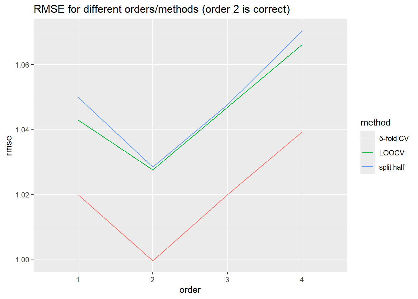
Table showing the final estimations of RMSE
df.rmse %>% group_by(method,order) %>% summarise(mean_rmse = mean(rmse)) %>% pivot_wider(names_from=order,values_from=mean_rmse)# A tibble: 3 × 5
# Groups: method [3]
method `1` `2` `3` `4`
<chr> <dbl> <dbl> <dbl> <dbl>
1 5-fold CV 1.02 1.000 1.02 1.04
2 LOOCV 1.04 1.03 1.05 1.07
3 split half 1.05 1.03 1.05 1.07Variance of Error Estimates
df.rmse %>% group_by(method,order) %>% summarise(var_rmse = var(rmse)) %>% pivot_wider(names_from=order,values_from=var_rmse)# A tibble: 3 × 5
# Groups: method [3]
method `1` `2` `3` `4`
<chr> <dbl> <dbl> <dbl> <dbl>
1 5-fold CV 0.0115 0.0109 0.0142 0.0148
2 LOOCV 0.0118 0.0142 0.0164 0.0154
3 split half 0.0123 0.0136 0.0151 0.0172Squared Bias of Error Estimates
options(scipen=999)
df.rmse$me <- modelErrors[df.rmse$order]
df.rmse %>% group_by(method,order) %>% summarise(bias2_rmse = mean(rmse-me)^2) %>% pivot_wider(names_from=order,values_from=bias2_rmse)
# A tibble: 3 × 5
# Groups: method [3]
method `1` `2` `3` `4`
<chr> <dbl> <dbl> <dbl> <dbl>
1 5-fold CV 0.00109 0.00155 0.00147 0.00137
2 LOOCV 0.0000982 0.000130 0.000131 0.000104
3 split half 0.00000816 0.000110 0.000113 0.000034835.7 A few key observations:
- Order 2 correctly found by both CV methods to be best order for fit (though k-fold tends to be more reliable on reruns)
- split half and LOOCV have higher variance in error estimates, 5-fold has lower variance.
- 5-fold tends to under-estimate model error, split in half over-estimates model error. The squared bias of split half is lower than either of the other two.