8  Random Variable Distribution Practice

9 Practice Problems

9.1 Using Wikipedia in college

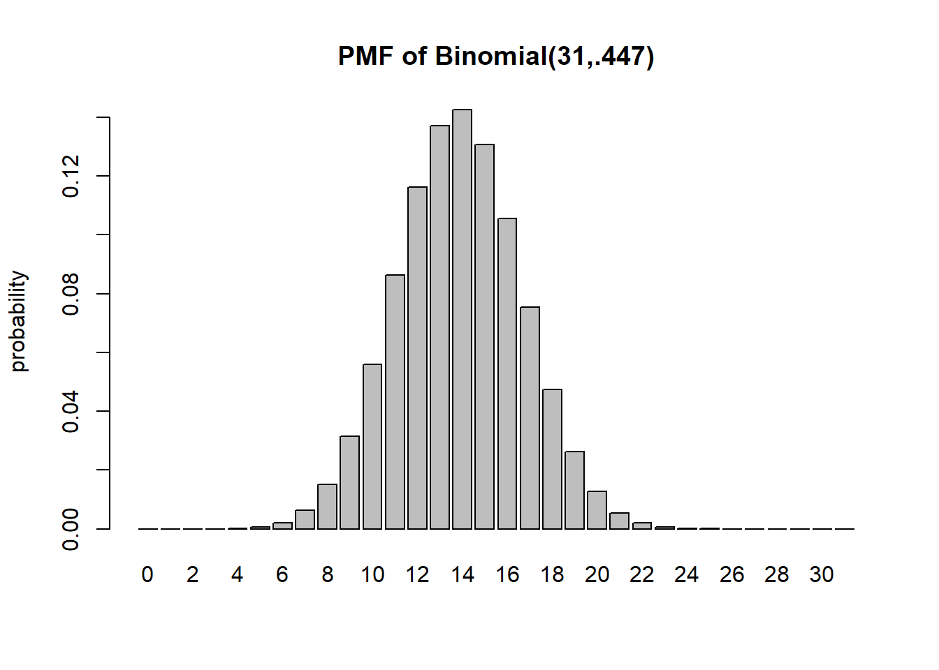
A recent national study showed that approximately 44.7% of college students have used Wikipedia as a source in at least one of their term papers. Let \(X\) equal the number of students in a random sample of size \(n = 31\) who have used Wikipedia as a source.

1. How is \(X\) distributed?

Solution

Assuming independence in sampling, and a representative sample, we can use a Binomial distribution with \(n=31\) and \(p=0.447\).

2. Sketch the probability mass function (roughly).

Solution

barplot(dbinom(0:31, 31,.447), names=0:31, ylab="probability", main="PMF of Binomial(31,.447)")

3. Sketch the cumulative distribution function (roughly).

Solution

plot(pbinom(0:31, 31, .447), type="s", ylab="cumulative prob.", main="CDF of Binomial(31, .447)")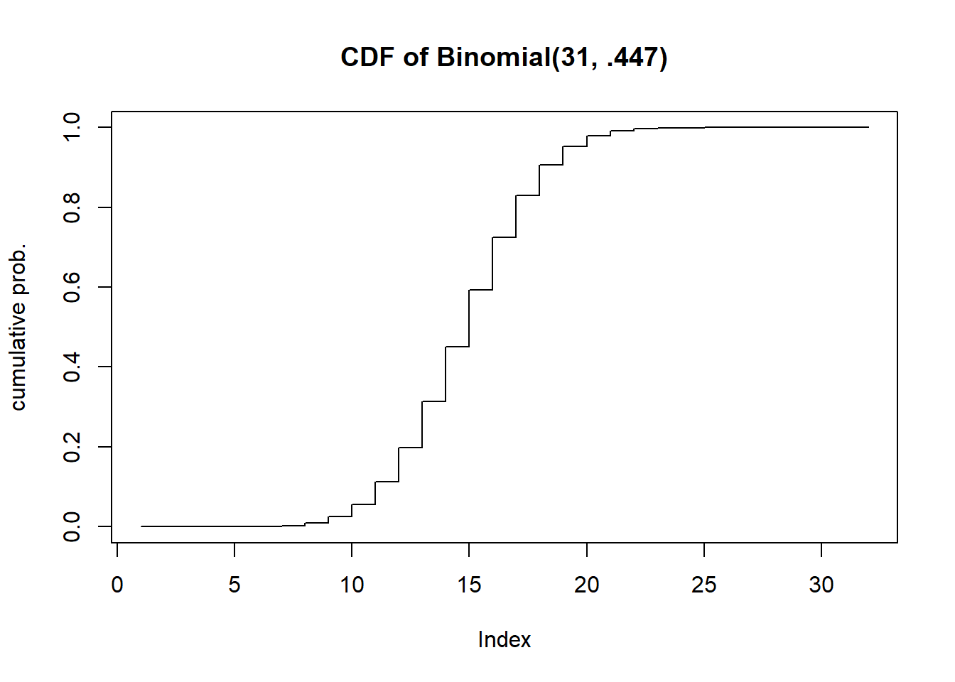

4. Find the probability that \(X\) is equal to 17.

Solution

dbinom(17, 31, .447)

[1] 0.07532248

5. Find the probability that \(X\) is at most 13.

Solution

pbinom(13, 31, .447)

[1] 0.451357

6. Find the probability that \(X\) is bigger than 11.

Solution

sum(dbinom(12:31, 31, .447))

[1] 0.8020339

#or
pbinom(11, 31, .447, lower.tail=FALSE)

[1] 0.8020339

#or
1-pbinom(11, 31, .447)

[1] 0.8020339

7. Find the probability that \(X\) is at least 15.

Solution

#P(X at least 15)
sum(dbinom(15:31,31,.447))

[1] 0.406024

8. Find the probability that \(X\) is between 16 and 19, inclusive.

Solution

sum(dbinom(16:19, 31, .447))

[1] 0.2544758

1. Give the mean of \(X\), denoted \(\mathbb{E}X\).

Solution

#E(X)=n*p
31*.447

[1] 13.857

#or you can also do this (but it's too much work)
sum( (0:31) * dbinom(0:31, 31, .447))

[1] 13.857

10. Give the variance of \(X\).

Solution

#Var(X) = n * p * (1-p)
31 * .447 * (1-.447)

[1] 7.662921

#or - if you want (but why would you want to?)
sum((0:31 - 31*.447)^2 * dbinom(0:31, 31, .447))

[1] 7.662921

11. Give the standard deviation of \(X\).

Solution

#SD(X) = sqrt(n*p*(1-p))
sqrt(31*.447*(1-.447))

[1] 2.768198

12. Find \(\mathbb{E}(4X+51.324)\).

Solution

#E(4X+51.324) = 4*E(X)+51.324
4*(31*.447) + 51.324

[1] 106.752

9.2 A Uniform PMF

Let \(X\) have discrete uniform PMF on the values \(x\in\left\{-1,0,1\right\}\).

1. Write the equation for its PMF.

2. Find \(Pr[X<-1]\) and \(Pr[X\leq -1]\)

3. Find \(Pr[X>0]\) and \(Pr[X \geq 0]\)

4. Calculate the CDF from the PDF. Write out an expression for \(F(x)\) and plot the PMF and CDF.

9.3 Discrete Random Variable Problems

1. If \(X\) is \(\text{Poisson}(\lambda)\), compute \(\mathbb{E}\left[1/(X+1)\right]\).

Solution

This can be handled mathematically. The formula for \(E(1/(X+1))\) is

\(E(1/(X+1))=\sum_{x=0}^{\infty}\frac{1}{x+1}\frac{\lambda^{x}}{x!}e^{-\lambda}=\sum_{x=0}^{\infty}\frac{\lambda^{x}}{(x+1)!}e^{-\lambda}\)

The trick is to get get the summation to equal 1 and simplify. We multiply by \(\lambda/\lambda\)

\(E(1/(X+1))=\frac{1}{\lambda}\sum_{x=0}^{\infty}\frac{\lambda^{x+1}}{(x+1)!}e^{-\lambda}\)

Now we can make a change of variables: \(y=x+1\) and thus \(x=0\) becomes \(y=1\)

\(E(1/(X+1)) = \frac{1}{\lambda}\sum_{y=1}^{\infty}\frac{\lambda^{y}}{y!}e^{-\lambda}\)

The only thing missing is that the summation starts at \(y=1\) instead of \(y=0\), But for \(Y \sim Poisson(\lambda)\), \(P(Y=0)=e^{-\lambda}\) so this summation is \(1-e^{-\lambda}\).

\(E(1/(X+1)) = \frac{1}{\lambda}(1-e^{-\lambda})\)

2. If \(X\) is \(\text{Bernoulli}(p)\) and \(Y\) is \(\text{Bernoulli}(q)\), computer \(\mathbb{E}\left[(X+Y)^3\right]\) assuming \(X\) and \(Y\) are independent.

Solution

\((X+Y)^3 = X^3+3X^2Y+3XY^2+Y^3\) so \(E[(X+Y)^3]=E(X^3)+3E(X^2)E(Y)+3E(X)E(Y^2)+E(Y^2)\)

this is due to independence. Since \(X\) an \(Y\) are independent, so are \(X^2\) and \(Y\), and \(X\) and \(Y^2\). \(E(X)=E(X^2)=E(X^3)=p\) and \(E(Y)=E(Y^2)=E(Y^3)=q\). Thus \(E[(X+Y)^3]=p+6pq+q\)

3. Let \(X\) be a random variable with mean \(\mu\) and variance \(\sigma^2\). Let \(\Delta(\theta)=\mathbb{E}\left[(X-\theta)^2\right]\). Find \(\theta\) that minimizes the error \(\Delta(\theta)\).

Solution

We can expand the expected value and attempt to find the minimum with respect to \(\theta\). \(E[(X-\theta)^2]=E[X^2-2\theta X+\theta^2]=E(X^2)-2\theta\mu+\theta^2\). Recall that \(Var(X)=E(X^2)-\mu^2\) so \(E(X^2)=\sigma^2+\mu^2\) So we can write \(\Delta(\theta)=\sigma^2 + \mu^2-2\theta\mu + \theta^2\) We want to find what value of \(\theta\) minimizes this function - derivative! \(\Delta'(\theta)=-2\mu+2\theta=0\) thus \(\theta=\mu\) minimizes this.

4. Suppose that \(X_1, \ldots, X_n\) are independent uniform random variables in \(\{0,1,\ldots,100\}\). Evaluate \(\mathbb{P}\left[\text{min}(X_1,\ldots, X_n) > l\right]\) for any \(l \in \{0,1,\ldots,100\}\).

Solution

Let \(Y=\min(X_1, \ldots, X_n)\) If \(P(Y >l)\), that means the minimum exceeds \(l\), so all of the values \(>l\). \(P(X_1 > l)=(100-l)/101\) - you can check: \(P(X_1>0)=100/101\). This is the same calculation for each \(i\). So \(P(Y>l)=\dfrac{(100-l)^n}{101^n}\).

5. Consider a binomial random variable \(X\) with parameters \(n\) and \(p\). \(p_X(k)={n \choose k} p^k(1-p)^{n-k}\). Show that the mean is \(\mathbb{E}X= np\).

Solution

\(E(X)=\sum_{k=0}^n k{n \choose k} p^k(1-p)^{n-k}\)

The first term is zero so we could write

\(\sum_{k=1}^n k{n \choose k} p^k(1-p)^{n-k}\)

Now the following is a fact that is needed but perhaps not well known. It’s the equivalence of \(k{n \choose k}=n{n-1 \choose k-1}\). We make this subsitution

\(\sum_{k=1}^n n{n-1 \choose k-1} p^k(1-p)^{n-k}=np\sum_{k=1}^n {n-1\choose k-1}p^{k-1}(1-p)^{n-k}\)

We could write \(n-k=(n-1)-(k-1)\) and we’ll be making some substitutions: \(m=n-1\) and \(j=k-1\). This lets us write

\(np\sum_{j=0}^m {m \choose j}p^j(1-p)^{m-j}=np\) because the summation =1, as it is just the sum of the pmf of a binomial.

6. (not for 340) Consider a geometric random variable \(X\) with parameter \(p\). \(p_X(k)=p(1-p)^k\) for \(k=0,1,\ldots\). Show that its mean is \(\mathbb{E}X=(1-p)/p\).

7. (not for 340) Consider a Poisson random variable \(X\) with parameter \(\lambda\). \(p_X(k)=\dfrac{\lambda^k}{k!}e^{-\lambda}\). Show that \(\text{Var}X=\lambda\).

8. (not for 340) Consider the uniform random variable \(X\) over values \(1,2,\ldots, L\). Show that \(\text{Var}X=\dfrac{L^2-1}{12}\). Hint: \(\sum_{i=1}^n i = \frac{n(n+1)}{2}\) and \(\sum_{i=1}^n i^2=\frac{n^3}{3}+\frac{n^2}{2}+\frac{n}{6}\)

9.4 Hard Drive Failures

An audio player uses a low-quality hard drive. The probability that the hard drive fails after being used for one month is 1/12. If it fails, the manufacturer offers a free-of-charge repair for the customer. For the cost of each repair, however, the manufacturer has to pay $20. The initial cost of building the player is $50, and the manufacturer offers a 1-year warranty. Within one year, the customer can ask for a free repair up to 12 times.

1. Let \(X\) be the number of months when the player fails. What is the PMF of \(X\)? Hint: \(\mathbb{P}(X = 1)\) may not be very high because if the hard drive fails it will be fixed by the manufacturer. Once fixed, the drive can fail again in the remaining months. So saying \(X = 1\) is equivalent to saying that there is only one failure in the entire 12-month period.

Solution

The number of failures should follow a binomial distribution with \(n=12, p=1/12\). Thus \(P(X=k)={n \choose k}(\frac{1}{12})^k(\frac{11}{12})^{n-k}\)

2. What is the average cost per player?

Solution

The cost is \(50+20X\) So \(E(50+20X)=50+20E(X)=50+20\cdot 12(\frac{1}{12})=70\)

9.5 Bit Errors

15. A binary communication channel has a probability of bit error of \(p = 10^{-6}\). Suppose that transmission occurs in blocks of 10,000 bits. Let \(N\) be the number of errors introduced by the channel in a transmission block.

1. What is the PMF of \(N\)?

Solution

\(N\) follows a binomial distribution with \(n=10000\) and \(p=.000001\)

2. Find \(\mathbb{P}(N = 0)\) and $(N b $ 3)$.

Solution

dbinom(0, 10000, .000001)

[1] 0.9900498

pbinom(3, 10000, .000001)

[1] 1

3. For what value of \(p\) will the probability of 1 or more errors in a block be 99%?

Solution

This can be solved directly. \(P(N \geq 1)=1-P(X=0)=1-(1-p)^{10000}\). If we set this to .99 we can solve for \(p\) : \(.99=1-(1-p)^{10000}\) so \(.01 = (1-p)^{10000}\) so \(p=1-.01^{1/10000}\)

1-.01^(1/10000)

[1] 0.000460411

9.6 Processing Orders

The number of orders waiting to be processed is given by a Poisson random variable with parameter \(\alpha = \frac{\lambda}{n\mu}\), where \(\lambda\) is the average number of orders that arrive in a day, \(\mu\) is the number of orders that an employee can process per day, and n is the number of employees. Let \(N; = 5\) and \(N< = 1\). Find the number of employees required so the probability that more than four orders are waiting is less than 10%.

Hint: You need to use trial and error for a few \(n\)’s.

Solution

lambda=5
mu=1
ppois(4, lambda/(1:10 * mu), lower.tail=FALSE)

 [1] 0.5595067149 0.1088219811 0.0275432568 0.0091242792 0.0036598468
 [6] 0.0016844329 0.0008589296 0.0004739871 0.0002784618 0.0001721156

#With 3 employees P(X>4) is less than 10%.

9.7 Normal Random Variable

If \(Z\sim \text{Normal}(\mu=0, \sigma^2=1^2)\) find

1. \(\mathbb{P}(Z > 2.64)\)

Solution

pnorm(2.64, 0, 1, lower.tail=FALSE)

[1] 0.004145301

2. \(\mathbb{P}(0 \leq Z < 0.87)\)

Solution

pnorm(.87)-pnorm(0)

[1] 0.3078498

3. \(\mathbb{P}(|Z| > 1.39)\) (Hint: draw a picture)

Solution

pnorm(1.39, lower.tail=FALSE)*2

[1] 0.1645289

9.8 Identify the Distribution

For the following random experiments, decide what the distribution of X should be. In nearly every case, there are additional assumptions that should be made for the distribution to apply; identify those assumptions (which may or may not strictly hold in practice).

1. We throw a dart at a dart board. Let X denote the squared linear distance from the bullseye to the where the dart landed.

Solution

Assume the dart lands somewhere on the board, and any point is equally likely (not a good assumption for a skilled dart thrower). The probability density would be proportional to the distance to the center squared - Suppose the dart board has radius \(R\). Let \(X\) be the distance to the dart from the bullseye. Then \(P(X<r)=\pi r^2 / (\pi R^2)=(r/R)^2\) . The question then is what is \(P(X^2<r)\)? Well, take a square root of both sides. \(=P(X < \sqrt{r})=\frac{r}{R^2}\). This is a uniform distribution’s CDF.

2. We randomly choose a textbook from the shelf at the bookstore and let P denote the proportion of the total pages of the book devoted to exercises.

Solution

A random proportion you might want to use uniform(0,1) however this is assuming that each proportion is equally likely. This is actually a great example for a beta distribution. Beta distributions are continuous distributions that can be parameterized to model a random proportion and the distribution can can be made to be skewed in different ways.

3. We measure the time it takes for the water to completely drain out of the kitchen sink.

Solution

Let’s assume the sink is filled to the maximum. We drain the sink and start our timer. In this case, it’s reasonable to model the length of time to drain as a normal distribution.

4. We randomly sample strangers at the grocery store and ask them how long it will take them to drive home.

Solution

The time it takes to go home could be modeled by a gamma distribution since it is a continuous distribution capped below at 0 and it is a useful way to model the length of time a random process takes to complete.

9.9 Normal Random Variable II

Let \(X\) be a Gaussian random variable with \(\mu=5\) and \(\sigma^2=16\).

1. Find \(\mathbb{P}(X>4)\) and \(\mathbb{P}(2\leq X \leq 7)\).

Solution

#P(X>4)
pnorm(4, mean=5, sd=4, lower.tail=FALSE)

[1] 0.5987063

#P(2 <= X <= 7)
pnorm(7, 5, 4)-pnorm(4,5,4)

[1] 0.2901688

2. If \(\mathbb{P}(X < a)=0.8869\), find \(a\).

Solution

qnorm(.88695, 4)

[1] 5.210466

3. If \(\mathbb{P}(X>b)=0.1131\), find \(b\).

Solution

qnorm(.1131, 5, 4, lower.tail=FALSE)

[1] 9.840823

4. If \(\mathbb{P}(13 < X \leq c)=0.0011\), find \(c\).

Solution

#First find the probability less than 13
p13 <- pnorm(13, 5, 4)
#now we can find the quantile for p13+.0011
qnorm(p13+.0011, 5, 4)

[1] 13.08321

#double check
pnorm(13.08321,5,4)-pnorm(13,5,4)

[1] 0.001100025

9.10 Choose the distribution

2. For the following situations, decide what the distribution of \(X\) should be. In nearly every case, there are additional assumptions that should be made for the distribution to apply; identify those assumptions (which may or may not hold in practice.)

1. We shoot basketballs at a basketball hoop, and count the number of shots until we make a basket. Let X denote the number of missed shots. On a normal day we would typically make about 37% of the shots.

Solution

The number of missed shots before the first basket, assuming independence, can be modeled by a Geometric random variable with parameter \(p=.37\).

2. In a local lottery in which a three digit number is selected randomly, let X be the number selected.

Solution

Assuming that all 3 digit numbers are equally likely (A reasonable assumption) the number selected can be modeled by a discrete uniform distribution with minimum 100 and maximum 999.

3. We drop a Styrofoam cup to the floor twenty times, each time recording whether the cup comes to rest perfectly right side up, or not. Let X be the number of times the cup lands perfectly right side up.

Solution

If we drop the cup 20 times, and the result each time is independent with a constant probability of landing right side up, the number of times it does can be modeled by a Binomial random variable with parameters \(n=20\) and \(p\) (unknown).

4. We toss a piece of trash at the garbage can from across the room. If we miss the trash can, we retrieve the trash and try again, continuing to toss until we make the shot. Let X denote the number of missed shots.

Solution

Geometric random variable (unknown parameter value for \(p\)).

5. Working for the border patrol, we inspect shipping cargo as when it enters the harbor looking for contraband. A certain ship comes to port with 557 cargo containers. Standard practice is to select 10 containers randomly and inspect each one very carefully, classifying it as either having contraband or not. Let X count the number of containers that illegally contain contraband.

Solution

Technically we should use a hypergeometric random variable for this situation (since it is a small population size of 557), but since we do not cover the hypergeometric the closest random variable we have is the binomial.

6. At the same time every year, some migratory birds land in a bush outside for a short rest. On a certain day, we look outside and let X denote the number of birds in the bush.

Solution

This is a discrete random variable, but without other information it’s hard to say. The distribution is likely unimodal and bell-curved. You could probably model this using a normal distribution rounded off to the nearest integer.

7. We count the number of rain drops that fall in a circular area on a sidewalk during a ten minute period of a thunder storm.

Solution

The observation window is the circular area, and the 10 minutes during observation. Assuming the rate of rainfall is constant, the number of raindrops in the circle can be modeled using a Poisson random variable.

8. We count the number of moth eggs on our window screen.

Solution

Counting indicates a discrete random variable. A binomial or a rounded normal distribution may be appropriate, but we lack enough details to be sure.

1. We count the number of blades of grass in a one square foot patch of land.

Solution

The location of the sprouting grass could be modeled well by a Poisson random variable - the \(\lambda\) parameter would likely be very large, in the range of 1000 or 10000, and as such the distribution would look very much like a normal distribution.

10. We count the number of pats on a baby’s back until (s)he burps.

Solution

As we define a geometric random variable, we let \(X\) be the number of failures before the first success. The last pat (that causes the burp) is the success in this context. So we could use a geometric random variable, but we would have to add 1 to it in order to count all burps (the failures + 1 success).

9.11 Two Normal RVs

Let X and Y be zero-mean, unit-variance independent Gaussian random variables. Find the value of r for which the probability that \((X, Y )\) falls inside a circle of radius r is 1/2.

Solution

x <- rnorm(10000)
y <- rnorm(10000)

r <- seq(1.1, 1.2, .005)
p <- 0
for (i in 1:length(r)){
  p[i] <- mean(sqrt(x^2+y^2) <= r[i])
}
data.frame(r,p)

       r      p
1  1.100 0.4525
2  1.105 0.4542
3  1.110 0.4568
4  1.115 0.4600
5  1.120 0.4622
6  1.125 0.4647
7  1.130 0.4690
8  1.135 0.4721
9  1.140 0.4754
10 1.145 0.4787
11 1.150 0.4818
12 1.155 0.4843
13 1.160 0.4869
14 1.165 0.4894
15 1.170 0.4920
16 1.175 0.4946
17 1.180 0.4975
18 1.185 0.5007
19 1.190 0.5032
20 1.195 0.5065
21 1.200 0.5089

#X^2 + Y^2 ~ Chisq(2)
#so the square root of the 50th percentile from that distribution should be the answer
sqrt(qchisq(.5,2))

[1] 1.17741

9.12 Uniform Random Angle

Let \(\Theta ∼ Uniform[0, 2\pi]\).

1. If \(X = cos \Theta\), \(Y = sin \Theta\). Are \(X\) and \(Y\) uncorrelated?

Solution

Yes, they are uncorrelated, because (x,y) can be any point on the circumference of a circle of radius 1 with uniform likelihood. However, they are not independent. If we know the value of \(Y\) for example, there are only 2 possible values of \(X\).

thetas <- runif(10000, 0, 2*pi)
cor(cos(thetas), sin(thetas))

[1] 0.0002646251

2. If \(X = cos(\Theta/4)\), \(Y = sin(\Theta/4)\). Are \(X\) and \(Y\) uncorrelated?

Solution

In this case (x,y) can only be found in the first quadrant. In this case they are going to be negatively correlated, since that portion of the unit circle in the first quadrant slopes downwards.

cor(cos(thetas/4), sin(thetas/4))

[1] -0.9183002

10 Beyond STAT 340

These problems are excellent practice but they are beyond the material we cover in STAT 340.

10.1 Variance of a Uniform RV

Calculate the variance of \(X \sim \text{Unif}(a,b)\). (Hint: First calculate \(\mathbb{E}X^2\))

10.2 Expectation and Binomial

If \(X \sim \text{Binom}(n,p)\) show that \(\mathbb{E}X(X-1)=n(n-1)p^2\).

Solution

We can just expand the product \(\mathbb{E}(X^2-X)\) and we can split this up into two expected values: \(\mathbb{E}X^2 - \mathbb{E}X = \mathbb{E}X^2-\mu\). Recall that \(Var(X)=\mathbb{E}X^2-\mu^2\) So \(\mathbb{E}X^2=Var(X)+\mu^2\). For a binomial, \(Var(X)=np(1-p)\) and \(\mu=np\). Thus we have

\(\mathbb{E}X^2 - \mu=[np(1-p) + n^2p^2] - np = np\left(1-p+np-1\right)\)

Tidying up a little bit we get \(np(np-p)=np^2(n-1)\), and we’re done.